
Note: A version of this paper has been published originally by Al Bento, "Tools for End-User Systems Development: a case example," Interface, Fall 1991, pp. 24-31. This is therefore copyrighted material. It is OK to read it here, link to it, but copying this page requires authorization from Interface and the author.
End-user systems development, and in specific decision support systems development, is one of the key factors for increasing productivity both in the end-user and in the MIS department environment. It decreases the demand for traditional systems development projects, and provides faster response to user needs. A key factor in promoting end-user systems development is the existence of friendly and 'MIS hygienic' end-user system development methodologies. In this paper a new approach for end-user systems development -- Management Through Information Systems -- is discussed, and a methodology for developing model oriented decision support systems using this approach is reviewed. Finally, a case for investment and price decisions is used as an example of DSS development using the MTIS approach, including implementation illustrations in Lotus 1-2-3.
1. INTRODUCTION
End-user systems development has been growing dramatically since the inception of PCs in the early 1980s [6,8,10]. One of the main types of systems developed by end-users is Decision Support Systems (DSS). DSS has a long history -- references are found as early as in the 1970s [11], but it is the introduction of PC hardware and software that makes DSS reach beyond the Planning departments, where primarily they had been developed [7].
End-user systems development has the potential for increasing productivity both in the end-user and in the MIS department environment. It provides faster response to user needs, and decreases the demand for traditional systems development projects.
A key factor in promoting end-user systems development is the existence of friendly and "MIS hygienic" end-user systems development methodologies. The need for supporting and controlling the risk involved in end-user systems development is much stressed in the literature [1,2,9,10,14].
The objective of this paper is to discuss and illustrate a methodology for end-user development of if-then decision support systems. The methodology presented here is part of a set of methodologies inspired by a new approach to end-user systems development, the "Management through Information Systems Approach" -- or, for short, the "MTIS Approach".
The MTIS approach broadens the traditional definition of management from "obtaining results through people" to "obtaining results through information systems", recognizing that managers, in all functional areas, are facing the challenge of combining people and computers to achieve the best results possible.
The MTIS approach, described in detail elsewhere [3], proposes different methodologies for systems development, according to the kind of managerial activity they are meant to support. According to this approach, Decision Support Systems are those that support the "steering activities," that is, all activities that change the existing ways of delivering goods and services in an organization, or that create new ones.
Steering activities can consist in a search for what the problem is, an analysis of possible alternatives to solve the problem, or a combination of both. Those three kinds of steering activities are supported, respectively, by three kinds of DSS: data-oriented (Data Analysis Models), model-oriented (If-Then Models) and both data and model oriented (Complex Models). This paper will exemplify the MTIS approach to the development of If-Then decision support systems. The purpose of If-Then DSS is to support iterative and interactive computation and comparison of alternatives.
In the model oriented steering activity the user/decision maker has three main tasks: (a) to build a model to structure the problem situation , (b) to identify, in this model, the factors and/or decisions he or she can manipulate to obtain a range of alternatives and (c) to compare the pros and cons of the range of alternatives thus generated.
The MTIS methodology for IF-Then DSS development addresses those tasks in two stages: (a) analysis, using influence diagram analysis and the requisite variety principle, and (b) design and implementation, using the variables-for-manipulation analysis, the dialog decision tree diagram, and the DSS generator specific implementation principle(s). Those two stages will be presented here on the basis of a case on investment and pricing decisions, using a widely known end-user language -- Lotus 1-2-3 -- as the DSS generator.
2. THE ABC CO. CASE
Mr. Know Hall, President of the ABC Co, is confronted with pricing and investment decisions for the next five years in the umbrella product line. He is concerned with the effect of these decisions on net after taxes and rate of return results.
Mr. Hall knows that by increasing investment in plant and equipments he can obtain a lower unit cost, but is uncertain of the effects on net after taxes and rate of return, because of the increased depreciation costs derived from new investments. He also knows that by increasing price he can obtain a higher margin, but is uncertain of the effects on results, because higher prices will decrease the sales volume. He figures that by manipulating these two variables he can find a combination that maximizes the product line results.
Mr. Hall decided to determine the effects of the sales price on volume, and investments on unit cost in a more precise way. He assigned to his assistant, Mr. E.T. Burn, the task of identifying these relations. Mr. Burn conducted a field test of price sensitivity by the umbrella customers, discussed the relationship of new machinery to unit prices with the manufacturing management and arrived to the following formulas:
VOLUME = 15,000 - 6,666 * SALES PRICE
UNIT COST = 1.3 - .00009 * INVESTMENT
Mr. Burn also pointed out that to estimate volume a market growth factor should be added to the formula, to account for the growth in the overall target population.
Mr. Hall decided to continue his analysis by trying to figure out the values of net after taxes and rate of return. He discovered that he needed ways to estimate manufacturing overhead and administrative expenses in order to finalize his model. Again Mr. Burn was assigned the task to look for these data. Analyzing the existing historical data Mr. Burn found that, in average, manufacturing overhead and administrative expenses were, respectively, 10% and 4% of net sales.
At this point Mr. Hall started to realize that figuring out by hand the net effect of sales price and investment in the results would be a very time consuming and repetitive task, if he decided to try various price and investment alternatives. He finally ordered Mr. Burn to buy a PC, Lotus 1-2-3, and develop a DSS to support the analysis of the problem.
3. MTIS ANALYSIS OF IF-THEN DSS
The objective of the DSS analysis process is to elicit the needs for computing alternatives and for showing the results in a meaningful context to the user, as well as, to access the data set required for these computations. The MTIS Analysis of If- Then decision support systems is based on influence diagram analysis and on application of the requisite variety principle.
Influence Diagram Analysis
The purpose of the analysis is to define a model to describe the decision situation, and to derive the corresponding data needs to support this model. The core methodology is the influence diagram [4] as a new and powerful tool to structure a decision situation, involving multiple relationships among variables at a single point in time.
The first activity to be performed is to prepare a narrative of the problem, including the purpose and reasons to pursue the analysis. The ABC Co. case write-up is an illustration of such a narrative.
The next activity is to identify and classify the variables involved in the decision situation. The variables can be classified in four basic types: (a) Decision variables: are controlled by the decision maker, and vary according to the alternatives selected; (b) Outcome variables: represent the results, or the measure of performance, effectiveness; (c) Exogenous/Assumption variables: are not determined in the model and/or must be taken for true; affect but are not affected by the other variable ; (d) Intermediate variables: are necessary to link decision and exogenous /assumption variables to outcome variables.
Table 1 shows the variables in the ABC case classified accordingly. It should be noted that the classification of variables depends upon how the user/decision maker sees the problem. For example, VOLUME is seen in the case as depending upon the SALES PRICE and MARKET GROWTH, while SALES PRICE is seen as a decision, and MARKET GROWTH as an exogenous variable. In a production steering decision problem, for example, VOLUME and SALES PRICE might be taken as exogenous, while some other variables might be defined as decisions, e.g., PLANT LOCATION.
VARIABLES CLASSIFICATION
| OUTCOME VARIABLES | NET AFTER TAX |
| RATE OF RETURN | |
| DECISION VARIABLES | SALES PRICE INVESTMENT |
| EXOGENOUS/ASSUMPTIONS VARIABLES | MKT GROWTH TAX RATE |
| INTERMEDIATE VARIABLES | VOLUME NET SALES UNIT COST DIRECT COSTS MFG OVERHEAD COST OF SALES GROSS PROFIT DEPRECIATION ADMIN EXPENSES NET BEFORE TAX |
The next activity is to draw the influence diagram. The influence diagram records the effect of a given variable on others, through simple graphic representations. A circle indicates a decision variable; a square identifies either an intermediate, or an exogenous/assumption variable; an ellipse represents an outcome variable; and an arrow indicates that one variable influences (affects) another. The general principle of drawing a influence diagram is to work backwards: start from the outcome variables and look for intermediate/exogenous variables until one reaches the decision variables.
Figure 1 shows the influence diagram for the ABC case. It should be noted again that the choice of what variables influence others is also dependent upon how the user/decision-maker sees the problem. For example, DEPRECIATION is shown affecting NET BEFORE TAX, while it might be seen affecting GROSS PROFIT, instead.
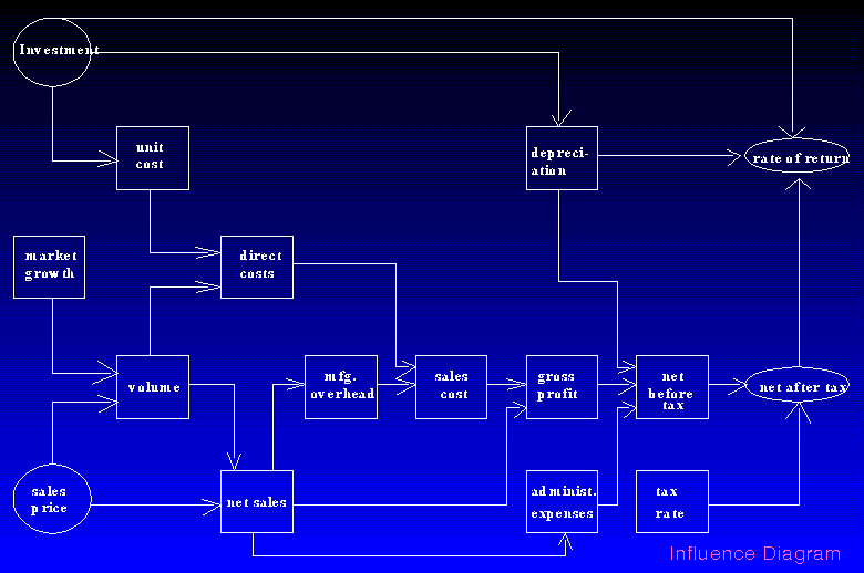
Figure 1: An Influence diagram for ABC
The next step in the method is to assign functional relations to the influence relations found (see Table 2). Most of the common models found in business practice are accounting-like, that is, linear in form. Other functional relations (exponential, logarithmic, logistic, hyperbolic) have also been used in business models.
EQUATIONS FOR SALES PRICE & INVESTMENT DECISIONS
VOLUME = 15,000 * (1 + MKT GROWTH) - 6,666 * SALES PRICE
UNIT COST = 1.3 - .00009 * INVESTMENT
NET SALES = SALES PRICE * VOLUME
DIRECT COSTS = UNIT COST * VOLUME
MFG OVERHEAD = .1 * NET SALES
COST OF SALES = MFG OVERHEAD + DIRECT COSTS
GROSS PROFIT = NET SALES - COST OF SALES
DEPRECIATION = FUNCTION (INVESTMENT)
ADMIN EXPENSES= .04 * NET SALES
NET BEFORE TAX= GROSS PROFIT - DEPRECIATION - ADMIN EXPENSES
NET AFTER TAX = (1- TAX RATE) * NET BEFORE TAX
RATE OF RETURN= FUNCTION (NET AFTER TAX+DEPRECIATION,INVESTMENT)
No functional form was specified for DEPRECIATION, nor RATE OF RETURN, since most of the DSS Generators possess the capabilities to compute these functions. This is valid for most of the financial, mathematical, and statistical functional forms.
Finally, the last activity is to determine the data needs. This is accomplished in a very simple way: the only variables that require data collection are the exogenous/assumption ones. This is so because outcome variables are computed as results of the model; decision variables are to be provided/manipulated by the user/decision maker; and intermediate variables are all determined by formulas in the model. Historical data for all the variables may also be required as a comparison with previous periods in time.
In the ABC case only data on MKT GROWTH and TAX RATE are required to be obtained externally to the model. In many situations the exogenous/assumption variables will constitute sets of environment scenarios in which the user/decision maker can evaluate the sensitivity of his decisions in regard to these same variables.
Application of the Requisite Variety Principle
In order to properly provide the requisite variety [5] for a DSS, output representations should be designed to compare the effect of different alternatives in intermediate and outcome variables. The number of possible comparisons and their types will depend upon the specific situation, but a comparison between three basic alternatives (worst, best, and expected cases) should always be provided.
In the ABC case six different alternative comparisons were provided, as shown in figure 2. For each of the alternatives shown in the final analysis, an infinite number of iterations takes place before they are selected to compare with others obtained in the same way.
 ----------------------------------------------------------------
                  1        2        3        4       5        6
 ----------------------------------------------------------------

 INVESTMENT     5,600    7,000    4,000    5,600   5,600    6,500

 SALES PRICE
    1985          1.5      1.5      1.5      1.7     1.3      1.6
    1986          1.5      1.5      1.5      1.7     1.3      1.6
    1987          1.5      1.5      1.5      1.5     1.5      1.6
    1988          1.5      1.5      1.5      1.3     1.7      1.6
    1989          1.5      1.5      1.5      1.3     1.7      1.6

 ----------------------------------------------------------------
 RATE OF RETURN 26.88%   27.16%   26.32%   23.73%  20.76%  27.65%
 ----------------------------------------------------------------
Figure 2 : Comparison of AlternativesThe output format for each individual alternative is shown in figure 3, in the part 4 of this work.
4. MTIS DESIGN AND IMPLEMENTATION OF IF-THEN DSS
The design stage corresponds to the mapping of information needs into software; the implementation stage refers to the actual coding, testing and documentation of the software. Both stages are highly connected in the DSS development process, given that there are no standards for DSS Generators, and therefore the design needs to take into consideration the specific features of a given DSS Generator.
In this work Lotus 1-2-3 was used as the DSS Generator for its simplicity and large penetration in the end-user community. Lotus 1-2-3 has a quite powerful Dialog Management System, with a strong and friendly presentation language -- the spreadsheet and the graphics -- based on the "input-in-context of output" principle [12], and increasingly powerful action language -- the macros. The Model Management System supports the implementation of accounting-like, financial, and basic statistic functions, and of what-if and sensitivity analysis. The Data Base Management System is the weakest part in the generator, but suffices the needs for developing IF-THEN DSS, for they do not require extensive data base functions.
The MTIS Design and Implementation of IF-THEN decision support systems is based on the variables-for-manipulation analysis, on the dialog decision trees diagrams, and on the implementation principles specific to the DSS Generator.
Variables-For-Manipulation Analysis
The model defined in the analysis stage is to be analyzed and the decision and/or exogenous/assumptions variables to be entered interactively should be identified. Auxiliary variables should be introduced in the equation to simplify the if-then manipulation. For example, instead of defining an equation like "UNITS SOLD = 50000, PREVIOUS UNITS SOLD * 1.05" (meaning fifty thousand units in the first period and the value of the units in the previous period increased by 5% thereafter), it should be defined as " UNITS SOLD=50000, PREVIOUS UNITS SOLD * (1 + GROWTH IN UNITS SOLD )," if the value of units sold is to be selected interactively by manipulating the growth rate. The variables-for-manipulation should be located in the same area of the model. This area should be identified as the only valid data entry area in the model.
In the ABC case the only variables to be manipulated are the UNIT PRICE and INVESTMENT, although at least MKT GROWTH could also have been chosen for this purpose. Figure 3 shows how our model/representation was implemented in Lotus 1-2-3. It should be noted that the structure shown in table 1, part 3, was maintained for illustration purposes only. In an actual situation we would have arranged the variables in a way that would match the user/decision-maker preferences. Nevertheless, the variables-for-manipulation would still be put together as in the example.
To prevent data entry in variables that are supposed to be computed by formulas, all entries in the spreadsheet were protected, except SALES PRICE (for all years), and INVESTMENT (for the first year). The protection was achieved using the command /Worksheet Global Protection Enable, and the unprotected cells were obtained using the command /Range Unprotect. After these commands, Lotus 1-2-3 shows in reverse video the areas where the data can be entered, and the word-wrap feature also works with the fields we unprotect to enter data, meaning that when the last entry is reached if we try to go any further the cursor moves to the first entry point again.
----------------------------------------------------------------
                       1985     1986     1987     1988     1989
----------------------------------------------------------------

DECISION VARIABLES

  SALES PRICE         $1.50    $1.50    $1.50    $1.50    $1.50
  INVESTMENT          5,600    5,600    5,600    5,600    5,600

----------------------------------------------------------------

ASSUMPTION VARIABLES

  MKT GROWTH           0.00%    5.00%    5.00%    3.00%    2.00%
  TAX RATE            46.00%   46.00%   46.00%   46.00%   46.00%

----------------------------------------------------------------

OUTCOME VARIABLES

  NET AFTER TAX       1,032    1,232    1,232    1,152    1,112
  RATE OF RETURN
    CASH FLOW        (4,008)   1,792    1,792    1,712    1,672
    RATE OF RETURN                                        26.88%

----------------------------------------------------------------

INTERMEDIATE VARIABLES

  VOLUME               5001     5751     5751     5451     5301
  UNIT COST           $0.80    $0.80    $0.80    $0.80    $0.80
  NET SALES           7,502    8,627    8,627    8,177    7,952
  DIRECT COST         3,981    4,578    4,578    4,339    4,220
  MFG OVERHEAD          750      863      863      818      795
  COST OF SALES       4,731    5,440    5,440    5,157    5,015
  GROSS PROFIT        2,771    3,186    3,186    3,020    2,937
  DEPRECIATION          560      560      560      560      560
  ADMIN EXPENSES        300      345      345      327      318
  NET BEFORE TAX      1,910    2,281    2,281    2,133    2,059

----------------------------------------------------------------
Figure 3 - Alternative Analysis Model/Representation
Dialog Decision Tree Diagrams
A decision tree is a graphical representation of a sequential, or multi-period, decision making process. As originally developed is composed of: decision points, alternatives, chance points, states of nature, and payoffs [13].
A dialog decision tree diagram is a graphical representation of the actions the user/decision maker can take, and what models and data sets are to be used to produce the results selected by the user action. Their basic elements are: decision points, alternatives, and actions. Figure 4 shows the usage of the dialog decision tree diagram for the ABC case. The squares indicate the decision points -- always in our example a combination of representations and menus, the circles indicate the actions -- what models and data should be used, and the arrows indicate the alternatives.
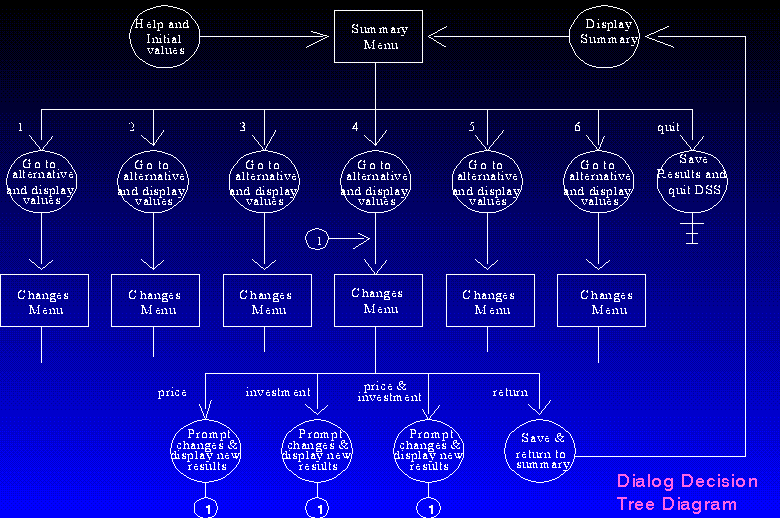
Figure 4: A dialog decision tree for ABC Co.
From another perspective the dialog decision tree diagram is the blueprint for the specific DSS action language, in our case, for the macros to be developed.
DSS Generator Specific Implementation Principles
Every DSS Generator has characteristics that can easily be perceived by the unprepared user as a 'trap'. These characteristics need to be analyzed and specific implementation principles need to be established before the dialog is coded. The purpose is to prevent errors to occur due to unforeseen consequences of otherwise apparently innocent actions.
In the case of Lotus 1-2-3 we should take into consideration that most of the actions we take have a row-wise or column-wise effect. If we insert a line or column in a spreadsheet, this will affect the whole spreadsheet and not only the part of the spreadsheet we are working on. This feature is prone to produce errors if we use more than one area of a given spreadsheet to define models, representations, and macros. The diagonal, the serial, or the 3-D specific implementation principles can be used to prevent these errors.
The diagonal approach (Figure 5a) prescribes that if we are to use more than one area of a spreadsheet then we should start the new area one or two cells to the bottom of the last row, and one or two cells to the right of the last column, and that cell (row and column) addresses be used to bind together all models. The serial approach (Figure 5b) prescribes that for every model a new spreadsheet should be used, and that macros should be used to bind together all models. The 3-D approach (Figure 5c) -- available for Lotus 1-2-3 releases 2.2 and 3.0 -- is a combination of both: every model should be created in a new spreadsheet, and cell (spreadsheet, row and column) addresses should be used to bind all models.

Figure 5: Lotus Implementation Principle
The advantage of the diagonal approach is that all models, macros,etc, are in the same spreadsheet, and therefore the consolidation or combination of files -- through the /File Combine command -- is avoided, decreasing the dialog/macros complexity. The disadvantage is the different cell addresses that each model (many times the same just adapted for a branch office or alternative) will have, increasing the possibility of referring to wrong cell addresses when consolidating spreadsheets, or comparing alternatives. Conversely, the advantage of the serial approach is to have the same cell addresses for all the models, while the disadvantage is a higher complexity level in the macro definitions.
The 3-D approach combines the advantages of the two other approaches, without their disadvantages, by adding to the cell address the spreadsheet name or address. The only known disadvantages are related to impact in performance: spreadsheets take a longer time to load and save, for the dynamic links among spreadsheets need to be updated.
The 3-D approach was used in the ABC case, using Lotus 3.1. Every alternative model/representation (figure 3) and the summary of alternatives (figure 2) were implemented as a spreadsheet. Three-dimensional (spreadsheet,row and column) addresses link the results of each alternative computation to the summary spreadsheet.
5. CONCLUSION
The purpose of this work was to discuss and illustrate a friendly and MIS hygienic methodology for the development of model oriented DSS. The MTIS concept and the MTIS Analysis and Design method for If-Then DSS were reviewed, and a detailed example of the usage of this method in the ABC Co. case was presented, including illustrations in the Lotus 1-2-3 end-user language.
The friendliness of the methodology is exemplified by the simplicity of the tools used, and by the step-by-step incremental solution of the decision-mechanic tasks, and their translation to an end-user language. Moreover, the method contributes to the problem solving activity, rather than just documenting it, helping the user/decision maker to define the alternatives and to define how to compare these alternatives.
The needs for end-user MIS hygienics are also supported by the method. All the tools used provide a standard and uniform way to develop and document every stage of the If-Then DSS, as well as to identify and protect user model formulas and data entry areas.
Finally, this work also calls the attention of practitioners and researchers for the need to develop methodologies oriented to specific DSS types, for the steering problems vary in nature.
1. Alavi, M. and Weiss, I.R. Managing the risks associated with end-user computing. Journal of MIS. 2, 3 (Winter 1985-86), 5-20.
2. Alavi, M., Nelson, R.R. and Weiss, I.R. End-user computing strategies: integrative framework. Journal of MIS. 4, 3 (Winter 1987-88), 28-49.
3. Bento, A.M. Management Through Information Systems: Decision Support Systems, Proceedings of HICSS-19, (January 1986), 379-388.
4. Bodily, S.E. Modern Decision Making .New York: McGraw-Hill, 1985, ch. 2-4.
5. Davis, G.B. and Olsen, M. Management Information Systems .New York: McGraw-Hill, 1985, 318-319.
6. Davis, F.D. Perceived usefulness, perceived ease of use, and user acceptance of information technology. MIS Quarterly, 13, 3 (September 1989), 319-339.
7. Hogue, J.T. and Watson, H.J. Management's role in the approval and administration of decision support systems. MIS Quarterly. 7, 2 (June 1983), 15-26.
8. Igbaria,M., Pavri, F.N. and Huff,S.L. Microcomputer applications: an empirical look at usage. Information and Management. 16, 4 (1989).
9. Morell, J.A. and Fleischer, M. Use of office automation by managers: how much, and to what purpose?. Information and Management. 14, 3 (1988), 205-210.
10. Munro, M.C., Huff, Sid L. and Moore, G. Expansion and control of end-user computing. Journal of MIS. 4, 3 (Winter 1987-88), 5-27.
11. Scott-Morton, M.S. Management decision systems: Computer based support for decision making. Division of Research, Harvard University, Cambridge, MA, 1971.
12. Sprague, R.H., and Carlson, E.D. Building Effective Decision Support Systems. Englewood Cliffs, NJ: Prentice-Hall, 1982.
13. Turban, E. and Meredith, J.R. Fundamentals of Management Science. Plano,Texas: Business Publications,Inc, 1985, 101-111.
14. Watson, H.J. and Carr, H.H. Organizing for dss support: end-user services. Journal of MIS. 4, 1 (Summer 1987), 83-95.