Excel Tutorial
In this textbook all of the examples are built around Excel. Our objective in this book is not to teach Excel (although this is a very valuable skill) but to teach problem-solving methods within Excel. We have found, however, that many students have trouble with quantitative methods because they are constantly struggling with Excel. Even students who know Excel reasonably well are often inefficient in doing simple, common tasks such as copying and pasting. For one thing, this can be frustrating to students when every task is tedious to perform. For another, it can greatly increase the time to perform tasks, especially in pressure environments such as during an exam!
Our purpose with this tutorial is to provide some Excel tips that will dramatically improve your efficiency. We concentrate on common tasks, not every last thing that can be done in Excel. Also, we presume that you have some Excel knowledge. We assume you know about rows and columns, values, labels, and formulas, relative and absolute addresses, and other basic Excel elements. If you know virtually nothing about Excel, you probably ought to work through an "Excel for Dummies" book and then work through this tutorial.
You can read this tutorial, or you can work through it in Excel. To do the latter, I suggest you print out this page.
Contents of this file
![]() Moving to the top of
the sheet
Moving to the top of
the sheet
![]() Copying and
pasting with the Special/Values option
Copying and
pasting with the Special/Values option
![]() Using
absolute/relative references
Using
absolute/relative references
![]() Inserting and
deleting rows or columns
Inserting and
deleting rows or columns
![]() Using the VLOOKUP
and HLOOKUP functions
Using the VLOOKUP
and HLOOKUP functions
![]() Creating range names
from labels
Creating range names
from labels
![]() Applying range
names in formulas
Applying range
names in formulas
![]() Using the same
range names in different sheets
Using the same
range names in different sheets
![]() Using Excel's
Tools/Options Menu Item
Using Excel's
Tools/Options Menu Item
Navigating in Excel
If everything in your spreadsheet fits on the screen, then you'll have no trouble moving around. But large spreadsheet models typically do not fit on the screen, so the ability to move around easily is a useful skill. Here are some handy tips.
Moving to the top of the sheet
Often you want to reorient yourself by going back to the "home" position on the worksheet. To go to the top left of the sheet (cell A1):
![]() Press Ctrl-Home (both keys at once).
Press Ctrl-Home (both keys at once).
Using End-arrow combinations
To go to the end of a range (top, bottom, left, or right):
![]() Press the End key, then the
appropriate arrow key. For example, press End and then right arrow to go to the
right edge of a range.
Press the End key, then the
appropriate arrow key. For example, press End and then right arrow to go to the
right edge of a range.
The action of an End-arrow combination depends on where you start. It takes you to the last nonblank cell if you start in a nonblank cell. (If there aren't any nonblank cells in that direction, it takes you to the far edge of the sheet.) If you start in a blank cell, it takes you to the first nonblank cell.
Splitting the screen
It is often useful to split the screen so that you can see more information. To split the screen vertically, horizontally, or both:
![]() Click on the narrow "screen
splitter" bar just to the right of the bottom scroll bar (for vertical
splitting) or just above the right-hand scroll bar (for horizontal splitting)
and drag this to the left or down.
Click on the narrow "screen
splitter" bar just to the right of the bottom scroll bar (for vertical
splitting) or just above the right-hand scroll bar (for horizontal splitting)
and drag this to the left or down.
Splitting gives you two "panes" (or four if you split in both directions). Once you have these panes, practice scrolling around in any of them, and see how the others react.
Selecting a range
In Excel, you usually select a range and then do something to it (such as enter a formula in it, format it, delete its contents, and so on). Therefore, it is extremely important to be able to select a range efficiently. It's easy if the whole range appears on the screen, but it's a bit trickier if you can't see the whole range. In the latter case the effect of dragging (the method most users try) can be frustrating---things scroll by too quickly. Try one of the following methods instead.
To select a range that fits on a screen:
![]() Click on one corner of the range and
drag to the opposite corner.
Click on one corner of the range and
drag to the opposite corner.
Or:
![]() Click on one corner, hold down the
Shift key, and click on the opposite corner.
Click on one corner, hold down the
Shift key, and click on the opposite corner.
To select a range doesn't fit on a screen:
![]() Click on one corner of the range, say,
the upper left corner. Then, holding the Shift key down, use the End-arrow
combinations (End and right arrow, then, if necessary, End and down arrow) to
get to the opposite corner.
Click on one corner of the range, say,
the upper left corner. Then, holding the Shift key down, use the End-arrow
combinations (End and right arrow, then, if necessary, End and down arrow) to
get to the opposite corner.
Or:
![]() Split the screen so that one corner
shows in one pane and the opposite corner shows in the other pane. Click on one
corner, hold the Shift key down, and click on the opposite corner.
Split the screen so that one corner
shows in one pane and the opposite corner shows in the other pane. Click on one
corner, hold the Shift key down, and click on the opposite corner.
Selecting multiple ranges
Sometimes you want to format more than one range in a certain way (as currency, for example). The quickest way is to select all ranges at once and then format them all at once. To select more than one range:
![]() Select the first range, press the Ctrl
key, select the second range, press the Ctrl key, select the third range, and
so on.
Select the first range, press the Ctrl
key, select the second range, press the Ctrl key, select the third range, and
so on.
For example, to select the ranges B2:D5 and F2:H5, click on B2, hold down the Shift key and click on D5 (so now the first range is selected), hold down the Ctrl key and click on F2, and finally hold down the Shift key and click on H5.
Common Operations
Copying and pasting
Copying and pasting (usually formulas) is one of the most frequently performed tasks in Excel, and it can be a real time-waster if done inefficiently. Many people do it as follows. They select the range to be copied (often in an inefficient manner), then they select the Edit/Copy menu item, then they select the paste range (again, often inefficiently), and finally they select the Edit/Paste menu item. There are much better ways to get the job done!
To copy and paste using keyboard shortcuts:
![]() Select the copy range (using one of
the efficient selection methods described above), press Ctrl-c (for copy),
select the paste range (again, efficiently), and press Ctrl-v (for paste). The
copy range will still have a dotted line around it. Press the Esc key to get
rid of it.
Select the copy range (using one of
the efficient selection methods described above), press Ctrl-c (for copy),
select the paste range (again, efficiently), and press Ctrl-v (for paste). The
copy range will still have a dotted line around it. Press the Esc key to get
rid of it.
To copy and paste using toolbar buttons:
![]() Proceed as above, but use the copy and
paste toolbar buttons (on the top toolbar) instead of the Ctrl-c and Ctrl-v key
combinations.
Proceed as above, but use the copy and
paste toolbar buttons (on the top toolbar) instead of the Ctrl-c and Ctrl-v key
combinations.
Buttons or key combinations? It's a matter of personal taste, but either is quicker than menu choices!
A frequent task is to enter a formula in one cell and copy it down a column or across a row. There are several very efficient ways to do this. To avoid copying and pasting altogether, use Ctrl-Enter:
![]() Starting with the top or left cell,
select the range where the results will go. (Use the selection methods
described earlier, especially if this range is a large one.) Type in the
formula, and press Ctrl-Enter instead of Enter.
Starting with the top or left cell,
select the range where the results will go. (Use the selection methods
described earlier, especially if this range is a large one.) Type in the
formula, and press Ctrl-Enter instead of Enter.
Pressing Ctrl-Enter enters what you typed in all of the selected cells (adjusted for relative addresses), so in general it can be a real time saver. For example, it could be used to enter the number 10 in a whole range of cells. Just select the range, type 10, and press Ctrl-Enter.
To copy with the drag handle:
![]() Enter the formula in the top or left
cell of the intended range. Place the cursor on the "drag handle" at
the lower right of this cell (the cursor becomes a plus sign), and drag this
handle down or across to copy.
Enter the formula in the top or left
cell of the intended range. Place the cursor on the "drag handle" at
the lower right of this cell (the cursor becomes a plus sign), and drag this
handle down or across to copy.
To copy by double-clicking on the drag handle:
![]() Enter the formula in the top or left
cell of the intended range. Double-click on the drag handle.
Enter the formula in the top or left
cell of the intended range. Double-click on the drag handle.
This latter method uses Excel's built-in intelligence, but it only works in certain situations. Let's say you have numbers in the range A3:B100. You want to enter a formula in cell C3 and copy it down to cell C100. Because this is a common thing to do, Excel does it for you if you double-click on the drag handle. It senses the "filled-up" range in column B and guesses that you want another filled-up range right next to it in column C. If there were no adjacent filled-up range, double-clicking on the drag handle wouldn't work.
Copying and pasting with the Special/Values option
Often you have a range of cells that contains formulas, and you would like to replace the formulas with the values they produce. Usually, you paste these values onto the copy range, that is, you overwrite the formulas with values. Alternatively, you could select another range for the paste range.
To copy formulas and paste values:
![]() Select the range with formulas, press
Ctrl-c to copy, and select the range where you want to paste the values (which
could be the same as the copy range). Then (because there is no keyboard
equivalent) select the Edit/Paste Special menu item, and select the Values
option.
Select the range with formulas, press
Ctrl-c to copy, and select the range where you want to paste the values (which
could be the same as the copy range). Then (because there is no keyboard
equivalent) select the Edit/Paste Special menu item, and select the Values
option.
You might want to experiment with the other options in the Edit/Paste Special dialog box. For example, if you have a set of labels entered as a row and you want this same set of labels entered somewhere else as a column, try copying and pasting special with the Transpose option. Or suppose you want to copy a cell's formula to another cell, but you do not want to copy the formatting of this cell. Then use the Formulas option.
Moving (cutting and pasting)
Often you would like to move information from one place in the sheet to another.
To move (cut and paste):
![]() Select the range to be cut, press
Ctrl-x (for cutting), select the upper left corner of the paste range, and
press Ctrl-v.
Select the range to be cut, press
Ctrl-x (for cutting), select the upper left corner of the paste range, and
press Ctrl-v.
As with copying and pasting, toolbar buttons can be used instead of key combinations, but either is more efficient than selecting menu items. Also, note that you need select only the upper left cell of the paste range. Excel knows that the shape of the paste range is the same as the shape of the cut range.
Using absolute/relative references
As you probably know, absolute and references are indicated in formulas by dollar signs or the lack of them, and they indicate what happens when you copy or move a formula to a range. You typically want some parts of the formula to stay fixed (absolute) and others to change relative to the cell position. This is a crucial concept for efficiency in spreadsheet operations, so you should take some time to understand it thoroughly. Here are two keys: (1) The dollar signs are relevant only for the purpose of copying or moving; they have no inherent effect on the formula. For example, the formulas =5*B3 and =5*$B$3 in cell C3, say, produce exactly the same result. Their difference is relevant only if cell C3 is copied or moved to some range. (2) There is never any need to type the dollar signs. This can be done with the F4 key.
To make a cell reference absolute or mixed absolute/relative using the F4 key:
![]() Enter a cell reference such as B3 in a
formula. Then press the F4 key.
Enter a cell reference such as B3 in a
formula. Then press the F4 key.
In fact, pressing the F4 key repeatedly cycles through the possibilities: B3 (neither row nor column fixed), then $B$3 (both column B and row 3 fixed), then B$3 (only row 3 fixed), then $B3 (only column B fixed), and back again to B3.
Inserting and deleting rows or columns
Often you want to insert or delete rows or columns. Note that deleting a row or column is not the same as clearing its contents--that is, making all its cells blank. Deleting means wiping it out completely.
To insert one or more blank rows:
![]() Click on a row number and drag down as
many rows as you want to insert, and then press Alt-i and then r (the menu
equivalent of Insert/Row).
Click on a row number and drag down as
many rows as you want to insert, and then press Alt-i and then r (the menu
equivalent of Insert/Row).
The rows you insert are inserted above the first row you selected. For example, if you select rows 8 through 11 and then insert, four blank rows will be inserted between the old rows 7 and 8. Columns are inserted in the same way, except that the key sequence is Alt-i and then c.
To delete one or more rows:
![]() Click on a row number and drag down as
many rows as you want to delete, and then press Alt-e and then d (the menu
equivalent of Edit/Delete).
Click on a row number and drag down as
many rows as you want to delete, and then press Alt-e and then d (the menu
equivalent of Edit/Delete).
Columns are deleted in exactly the same way.
Filling a series
Say you want to fill column A, starting in cell A2, with the values 1, 2, and so on up to 1000. There is an easy way.
To fill a column range with a series:
![]() Enter the first value in the first cell
(1 in cell A2). With the cursor in the starting cell (A2), use the
Edit/Fill/Series menu item to obtain a dialog box. Change the Row setting to
Column, enter 1 in the Step Value box, enter the final value (1000) in the Stop
Value box, and click on OK.
Enter the first value in the first cell
(1 in cell A2). With the cursor in the starting cell (A2), use the
Edit/Fill/Series menu item to obtain a dialog box. Change the Row setting to
Column, enter 1 in the Step Value box, enter the final value (1000) in the Stop
Value box, and click on OK.
As you can guess from this dialog box, many other options are possible, but we have found the above set of options to be the most useful.
Using Formulas and Functions
Common functions
There are many useful functions in Excel. You should become familiar with the ones most useful to you (for example, financial analysts should learn the financial functions), but here are a few everyone should know. (By the way, we capitalize the names of these functions just for emphasis. They are not case sensitive. You can enter SUM, Sum, sum, or even sUM, with the same result.)
![]() Enter the formula =SUM(range),
where range is any range. This sums the numerical values in the
range. It ignores nonnumerical values (or blank cells) in the range.
Enter the formula =SUM(range),
where range is any range. This sums the numerical values in the
range. It ignores nonnumerical values (or blank cells) in the range.
Actually, it is possible to include more than one range in a SUM formula if the ranges are separated by commas. (This can also be done with the COUNT, COUNTA, AVERAGE, MAX, and MIN functions discussed below.) For example, =SUM(B5,C10:D12,Revenues) is allowable (where Revenues is a name for some range). The result is the sum of the numerical values in all of these ranges combined.
![]() Enter the formula =AVERAGE(range)
where range is any range. This produces the average of the numerical
values in the range. It ignores nonnumerical values in the range.
Enter the formula =AVERAGE(range)
where range is any range. This produces the average of the numerical
values in the range. It ignores nonnumerical values in the range.
Be aware that the AVERAGE function ignores labels and blank cells in the average. So, for example, if the range C3:C50 includes scores for students on a test, but cells C6 and C32 are blank because these students haven't yet taken the test, then =AVERAGE(C3:C50) averages only the scores for the students who took the test. It does not automatically average in zeros for the two who didn't take the test.
![]() Enter the formula =MAX(range)
or =MIN(range) where range is any range. These produce the
obvious results: the maximum (or minimum) value in the range.
Enter the formula =MAX(range)
or =MIN(range) where range is any range. These produce the
obvious results: the maximum (or minimum) value in the range.
![]() Enter the formula =COUNT(range),
where range is any range. This produces the number of numerical
values in the range. It ignores nonnumerical values in the range.
Enter the formula =COUNT(range),
where range is any range. This produces the number of numerical
values in the range. It ignores nonnumerical values in the range.
There is a similar function, COUNTA, that counts all of the cells, numerical or nonnumerical, in the range(s). For example, if cells A1, A2, and A3 contain Month, 1, and 2, respectively, then =COUNT(A1:A3) yields 2, whereas =COUNTA(A1:A3) yields 3.
Often you want to count the number of values in a range that satisfy a certain condition. Then you can use the COUNTIF function.
![]() Enter the formula =COUNTIF(range,
condition) where range is any range and condition is a
condition that is either true or false for every cell in the range.
Enter the formula =COUNTIF(range,
condition) where range is any range and condition is a
condition that is either true or false for every cell in the range.
For example, suppose you have employee salaries in the range B4:B301 and you want to know how many of these employees earn more than $50,000. Then you can use the formula =COUNTIF(B4:B301,">50000"), where the quotes around the condition are necessary. If the cutoff number, 50000, happens to be in a cell B2, you can refer to it with the following syntax: =COUNTIF(B4:B301,">"&B2).
Using the summation button
The SUM function is used so often to sum across rows or columns that a toolbar button (the S button) is available to automate the procedure. To illustrate its use, suppose you have a table of numbers in the range B3:E7. You want the row sums to appear in the range F3:F7, and you want the column sums to appear in the range B8:E8. It's easy.
To produce row and column sums with the summation button:
![]() Select the range(s) where you want the
sums (F3:F7 and B8:E8---remember how to select multiple ranges) and click on
the summation button.
Select the range(s) where you want the
sums (F3:F7 and B8:E8---remember how to select multiple ranges) and click on
the summation button.
Note that if you select multiple cells, you get the sums automatically. If you select a single cell (such as when you have a single column of numbers to sum), you'll be shown the sum formula "for your approval" and you'll have to press Enter to actually enter it. Why does Excel do it this way---who knows?
Using the SUMPRODUCT function
Everyone knows the SUM function, but most people don't know the SUMPRODUCT function, a function that is frequently used in this book. As its name implies, it forms a sum of products, as in 3(5)+6(4)+2(7)=53.
To enter a SUMPRODUCT function:
![]() Enter the formula =SUMPRODUCT(range1,
range2) where range1 and range2 are any ranges with exactly
the same size and shape.
Enter the formula =SUMPRODUCT(range1,
range2) where range1 and range2 are any ranges with exactly
the same size and shape.
For example, the formula =SUMPRODUCT(B1:B3,C17:C19) is equivalent to the formula =B1*C17+B2*C18+B3*C19. You might prefer the latter for this particular example, but try writing out =SUMPRODUCT(B1:B100,C17:C116) and you'll appreciate the usefulness of the SUMPRODUCT function. Note that the formula =SUMPRODUCT(B1:B3,C17:E17) will produce an error. Each of these ranges has 3 cells, but the cells in the first range go down a column, whereas the cells in the second go across a row. The two ranges must have exactly the same shape.
Using the IF function
IF functions are very useful, and they vary from simple to very complex. We'll provide a few examples.
To enter a basic IF function:
![]() Enter the formula =IF(condition,
expression1, expression2), where condition is any
condition that is either true or false, expression1 is the value of the
formula if the condition is true, and expression2 is the value of the
formula if the condition is false.
Enter the formula =IF(condition,
expression1, expression2), where condition is any
condition that is either true or false, expression1 is the value of the
formula if the condition is true, and expression2 is the value of the
formula if the condition is false.
A simple example is =IF(A1<5,10,"NA"). Note that if either of the expressions is a label (as opposed to a numerical value), it should be enclosed in double quotes.
Sometimes IF functions are nested. For example, suppose there are three outcomes, depending on whether the value in cell A1 is negative, zero, or positive. A nested IF formula could then be used as follows.
To use nested IF functions:
![]() Enter the formula =IF(condition1,expression1,IF(condition2,expression2,
expression3)). If condition1 is true, the relevant value is expression1.
Otherwise, condition2 is checked. If it is true, the relevant value is expression2.
Otherwise, the relevant value is expression3.
Enter the formula =IF(condition1,expression1,IF(condition2,expression2,
expression3)). If condition1 is true, the relevant value is expression1.
Otherwise, condition2 is checked. If it is true, the relevant value is expression2.
Otherwise, the relevant value is expression3.
An example is =IF(A1<0,10,IF(A1=0,20,30)). Suppose this formula is entered in cell B2. Then if A1 contains a negative number, B2 contains 10. Otherwise, if A1 contains 0, B2 contains 20. Otherwise (meaning that A1 must contain a positive value), B2 contains 30. The hardest thing about nested IF formulas is getting the right number of parentheses in the right places!
Sometimes more complex conditions (AND or OR conditions) are useful in IF functions. These are not difficult once you know the syntax.
To use an AND condition in an IF function:
![]() Enter the formula =IF(AND(condition1,
condition2), expression1, expression2). This results in expression1
if both condition1 and condition2 are true. Otherwise, it results
in expression2.
Enter the formula =IF(AND(condition1,
condition2), expression1, expression2). This results in expression1
if both condition1 and condition2 are true. Otherwise, it results
in expression2.
Note the syntax. The keyword AND is followed by the conditions, separated by a comma and enclosed within parentheses. Of course, more than two conditions could be included in the AND.
To use an OR condition in an IF function:
![]() Enter the formula =IF(OR(condition1,
condition2), expression1, expression2). This results in expression1
if either condition1 or condition2 is true (or if they're both
true). Otherwise, it results in expression2.
Enter the formula =IF(OR(condition1,
condition2), expression1, expression2). This results in expression1
if either condition1 or condition2 is true (or if they're both
true). Otherwise, it results in expression2.
Again, more than two conditions could be included in the OR.
You might not do it often, but you can mix AND and OR conditions. An example is =IF(OR(B1="Jan",AND(A1=1999,B1="Feb")),5,10). In this example, if B1 contains Jan, or if A1 contains 1999 and B1 contains Feb, the result is 5. In all other cases, the result is 10. Again, the hardest part is getting the parentheses straight.
Using the VLOOKUP and HLOOKUP functions
Lookup tables are useful when you want to compare a particular value to a set of values, and depending on where your value falls, return a given "answer." For example, you might have a tax table that shows, for any gross adjusted income, what the corresponding tax is. There are two versions of lookup tables, vertical (VLOOKUP) and horizontal (HLOOKUP). Becuase they are virtually identical except that vertical goes down whereas horizontal goes across, we'll discuss only the VLOOKUP function.
The VLOOKUP function takes three arguments: (1) the value to be compared, (2) a table of lookup values, with the values to be compared against always in the leftmost column in ascending order, and (3) the column number of the lookup table where you find the "answer." Because the VLOOKUP function is often copied down a column, it is usually necessary to make the second argument an absolute reference, and this is accomplished most easily by giving the lookup table a range name such as LTable. (Range names are always treated as absolute references.)
Let's say you want to assign letter grades to students based on a straight scale: below 60, an F: at least 60 but below 70, a D; at least 70 but below 80, a C; at least 80 but below 90, a B; and 90 or above, an A. Then the left column of the lookup table should contain the values 0, 60, 70, 80, and 90, in that order. The labels in the second column are then F, D, C, B, and A. If a student scores 77, this score is compared to the first column in the lookup table. Because 70 is the first value less than or equal to 77, the student receives a C.
To use a VLOOKUP function:
![]() Create a lookup table with at least
two columns, where the values in the first column are in ascending order, and
(for best results) give the table range a range name. Then enter the formula
=VLOOKUP(Value,LookupTable,Column #), as described above.
Create a lookup table with at least
two columns, where the values in the first column are in ascending order, and
(for best results) give the table range a range name. Then enter the formula
=VLOOKUP(Value,LookupTable,Column #), as described above.
As an example, if you enter =VLOOKUP(B7,LTable,3), Excel compares the value in B7 to the first column of the lookup table (range-named LTable) and returns the corresponding value from the third column of the lookup table.
Using the NPV function
There are many financial functions in Excel, but the one we will use most often is the net present value (NPV) function. The purpose of this function is to convert a stream of revenues and/or costs that occur through time into a single equivalent present value. We say that we discount these revenues and costs back to the present time.
To use the NPV function:
![]() Enter the formula =NPV(discount
rate, range), where discount rate is the relevant discount
rate, and range is a range that contains the monetary values.
Enter the formula =NPV(discount
rate, range), where discount rate is the relevant discount
rate, and range is a range that contains the monetary values.
The discount rate is relative to the timing. For example, if the range contains monthly revenues, then the discount rate should be a monthly rate. Timing is also important for the values in the monetary range. We assume that these values occur at the ends of period 1, period 2, and so on. If the first value in the range really occurs at the beginning of period 1, then it should be pulled outside of the NPV function. For example, if a company pays $1000 at the beginning of month 1 and then receives revenues $600 and $700 at the ends of months 1 and 2, and if these monetary values are in the range B20:B22, then the NPV can be found with the formula =NPV(0.01,B21:B22)-B20 (assuming a 1% discount rate per month).
Using the function wizard (fx) button in the top toolbar
If you haven't used this button, you should give it a try. It not only lists all of the functions available in Excel (by category), but it also leads you through the use of them. As an example, suppose you know there is an Excel function that does net present value, but you can't remember its name is or how to use it. You could proceed as follows.
To use the function wizard:
![]() Select a blank cell where you want the
formula to go. Press the fx button and click on the category that
seems most appropriate (in this case, Financial). Scan through the list for a
likely candidate and select it (try NPV). At this point you can get help, or
you can press the Next button and enter the appropriate arguments for the
function (discount rate and one or more ranges of monetary values).
Select a blank cell where you want the
formula to go. Press the fx button and click on the category that
seems most appropriate (in this case, Financial). Scan through the list for a
likely candidate and select it (try NPV). At this point you can get help, or
you can press the Next button and enter the appropriate arguments for the
function (discount rate and one or more ranges of monetary values).
Sometimes Excel add-ins create functions that are not built into Excel. If these add-ins are loaded, then you can see their functions with the function wizard by selecting the User Defined category. This is relevant for the StatPro, RandFns, and @Risk add-ins used in this book.
Range Names
Range names are extremely useful for making your formulas more understandable. After all, which formula makes more sense: =B20-B21 or =Revenue-Cost? Efficient use of range names takes some experience, but here are a few useful tips.
Creating range names
To create a range name:
![]() Select a range that you want to name.
Then type the desired range name in the upper left "name box" on the
screen. This box is just above the column A heading. It usually shows the cell
address, such as E13, where the cursor is. Just highlight this cell address,
type your range name over it, and press Enter. (Don't forget to press Enter.
Otherwise, you'll have to do it all over again.)
Select a range that you want to name.
Then type the desired range name in the upper left "name box" on the
screen. This box is just above the column A heading. It usually shows the cell
address, such as E13, where the cursor is. Just highlight this cell address,
type your range name over it, and press Enter. (Don't forget to press Enter.
Otherwise, you'll have to do it all over again.)
You can also go through the Insert/Name/Define menu item to create range names, but typing in the name box is quicker and more intuitive. By the way, range names are not case sensitive. For example, Revenue, revenue, and REVENUE can be used interchangeably.
Deleting range names
To delete a range name:
![]() Use the Insert/Name/Define menu item.
This shows a list of all range names in your workbook. Click on the one you
want to delete, and then click on the Delete button.
Use the Insert/Name/Define menu item.
This shows a list of all range names in your workbook. Click on the one you
want to delete, and then click on the Delete button.
Creating range names from labels
Suppose you have the labels Revenue, Cost, and Profit in cells A20, A21, and A22, and you would like the cells B20, B21, and B22 (which will contain the values of revenue, cost, and profit) to have these range names. Here's how to do it quickly.
To create range names from adjacent labels:
![]() Select the range consisting of the
labels and the cells to be named (A20:B22). Then use the
Insert/Name/Create menu item, make sure the appropriate box (in this case, Left
Column) is checked, and click on OK.
Select the range consisting of the
labels and the cells to be named (A20:B22). Then use the
Insert/Name/Create menu item, make sure the appropriate box (in this case, Left
Column) is checked, and click on OK.
Excel tries (usually successfully) to guess where the labels are that you want to use as range names. If it guesses incorrectly, you can always override its guesses.
Applying range names in formulas
Sometimes you have entered a formula using cell addresses, such as =B20-B21. Later, you name B20 as Revenue and B21 as Cost. The formula does not change to =Revenue-Cost automatically. However, you can make it change (and hence become more readable).
To apply range names to an existing formula:
![]() Select the cell (or range of cells)
with the formula(s). Then use the Insert/Name/Apply menu item, highlight any
relevant range names for the formula(s) involved, and click on OK.
Select the cell (or range of cells)
with the formula(s). Then use the Insert/Name/Apply menu item, highlight any
relevant range names for the formula(s) involved, and click on OK.
Getting a list of range names
If you have defined a lot of range names, it is sometimes useful to see a list of them, along with the ranges to which they apply.
To see a list of all range names and the ranges to which they apply:
![]() Click on the down arrow at the right
of the name box, and click on any of the range names you see. That range will
then be selected automatically.
Click on the down arrow at the right
of the name box, and click on any of the range names you see. That range will
then be selected automatically.
You can also paste a list of range names and their corresponding cell addresses into your sheet. To do so:
![]() Select a cell where you want the list
to be pasted. Then use the Insert/Names/Paste menu item, and click on the Paste
List button.
Select a cell where you want the list
to be pasted. Then use the Insert/Names/Paste menu item, and click on the Paste
List button.
Using range names in formulas
It is usually straightforward to use range names in formulas. For example, if B20 is named Revenue and B21 is named Cost, then entering the formula =Revenue-Cost in cell B22 is a natural thing to do. But consider this situation. The range B3:B14 contains revenues for each of 12 months, and its range name is Revenues. Similarly, C3:C14 contains monthly costs, and its range name is Costs. For each month, you want that month's revenue minus cost in the corresponding cell in column D. You will get it correct if you select the range D3:D14, type the formula =Revenues-Costs, and press Ctrl-Enter. If you click on any cell in this range, you'll see the formula =Revenues-Costs.
This can be confusing. How does Excel know that the formula in D3, for example, is really =B3-C3? Let's just say that Excel is smart enough to figure this out. If it confuses you, however, you can always enter =B3-C3 and copy it down. Then you're safe, but you've lost the advantage of range names. (We always do it this "simple" way in our examples because we usually get confused by trying to be too clever!)
Using the same range names in different sheets
Multisheet Excel files can be really tricky when it comes to range names. Suppose you have a file with two sheets named Sheet1 and Sheet2. You give the range A1:A10 on Sheet 1 the name Costs. Then you can refer to this range name in a formula in either Sheet1 or Sheet2. So far, so good. However, what if you also want to create a Costs range name for a range in Sheet2. Here's where things get tricky.
The best way to do this is to precede the range names with the sheet name when you define them. Specifically, use the range name Sheet1!Costs for the range in Sheet1, and use the name Sheet2!Costs for the range in Sheet2. Now suppose you want to enter a formula in Sheet2 that subtracts the sum of the costs on Sheet2 from the sum of the costs on Sheet1. Then you could use either of the formulas =SUM(Sheet1!Costs)-SUM(Sheet2!Costs) or =SUM(Sheet1!Costs)-SUM(Costs). Because this formula is on Sheet2, Excel figures that Costs, without a sheet reference, refers to the Sheet2 Costs range.
To create a "sheet-level" range name:
![]() Enter the range name in the "name
box" in the usual way, but precede it with the sheet name and an
exclamation point, as in Sheet1!Costs.
Enter the range name in the "name
box" in the usual way, but precede it with the sheet name and an
exclamation point, as in Sheet1!Costs.
Using Data Tables
Data tables, also called what-if tables, allow you to see very quickly how one or more outputs change as one or two key inputs change. There are two types of data tables: one-way tables and two-way tables. A one-way table has one input and any number of outputs. A two-way table has two inputs but only one output. We'll demonstrate both types.
Creating one-way tables
To illustrate, suppose Mr. Jones buys a new car for $15,000, makes a $3,000 down payment, and finances the remaining amount over the next 36 months at an 12% annual interest rate. There are at least two outputs that might be of interest: the monthly payment and the total interest paid. These are affected by at least two inputs: the amount of the down payment and the term (number of payments).
Let's first look at a simple "one-way" data table, where we see how a single output, monthly payment, varies as the down payment varies. This is shown in rows 21-27 of the following figure.
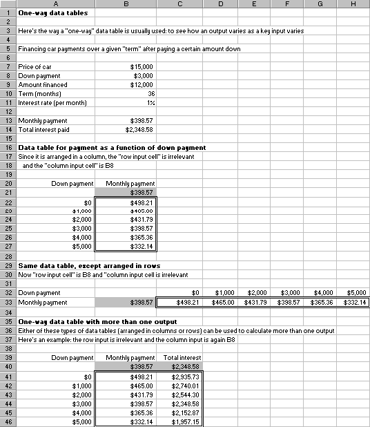
To create this table:
![]() First, create the model through row
14. Note that the interest rate in cell B11 is a monthly rate, the annual rate
divided by 12. Then the outputs in cells B13 and B14 are calculated with the
formulas =PMT(B11,B10,-B9) and =B10*B13-B9.
First, create the model through row
14. Note that the interest rate in cell B11 is a monthly rate, the annual rate
divided by 12. Then the outputs in cells B13 and B14 are calculated with the
formulas =PMT(B11,B10,-B9) and =B10*B13-B9.
![]() Create a link in cell B21 to the
output in cell B13 with the formula =B13.
Create a link in cell B21 to the
output in cell B13 with the formula =B13.
![]() Highlight the range A21:B27, use the
Data/Table menu item, leave the Row Input Cell box blank, enter B8 (the down
payment cell) in the Column Input Cell box, and click on OK.
Highlight the range A21:B27, use the
Data/Table menu item, leave the Row Input Cell box blank, enter B8 (the down
payment cell) in the Column Input Cell box, and click on OK.
When you do this, Excel takes each down payment value in the A22:A27 range, substitutes it into the column input cell you chose (cell B8), recalculates the formula in cell B21 (the one we colored gray for emphasis) with this new down payment, and records the answer in the data table. We use a column input cell because the possible inputs (down payments) are listed in a column.
The data table in rows 32 and 33 is exactly the same except that it goes across rows, not down columns. Here we use cell D8 as the Row Input Cell, and we don't enter a Column Input Cell.
We can also capture more than one output in a one-way data table. An example appears in rows 40-46, where the single input is still the down payment, but there are two outputs: monthly payment and total interest paid. This table is formed exactly as the first data table except that the table range is now A40:C46.
Creating two-way data tables
Two-way tables allow you to vary two inputs, one along a row and one along a column, and capture a single output in the body of the table. The following figure illustrates this in rows 19-25, where we vary the term and the amount of the down payment. The single output is the monthly payment.
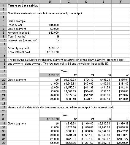
To create this table:
![]() Enter the formula =B12 for the single
output in the upper left corner (cell B19) of the data table. (Again, we color
this cell gray for emphasis.)
Enter the formula =B12 for the single
output in the upper left corner (cell B19) of the data table. (Again, we color
this cell gray for emphasis.)
![]() Enter any sequence of terms to the
right of this and any sequence of down payments below this.
Enter any sequence of terms to the
right of this and any sequence of down payments below this.
![]() Finally, select the entire data table
range, B19:F25, use the Data/Table menu item, enter B9 as the row input cell,
and enter B7 as the column input cell.
Finally, select the entire data table
range, B19:F25, use the Data/Table menu item, enter B9 as the row input cell,
and enter B7 as the column input cell.
Note that B9 is the row input cell because various terms are entered in row 19. Similarly, B7 is the column input cell because various down payments are entered in column B. Excel substitutes each term into cell B9 and each down payment into cell B7, calculates the formula in cell B19, and records the answer (monthly payment) in the body of the table.
If we want to see how another output varies as these two inputs vary, we have to create another two-way data table, as the above figure shows in rows 30-36. The only difference is that we now create a link to the total interest paid by entering the formula =B13 in cell B30.
The Goal Seek Tool
When we study optimization in Chapters 14 and 15, we learn a lot about Excel's powerful Solver add-in. A much less powerful, but still useful, tool is Excel's built-in Goal Seek. Essentially, it is useful for solving one equation in one unknown. As an example, suppose we create an Excel model for a company's profit. Although several inputs are used to drive profit, one of them that we're particularly interested in is the unit price to charge for the product. This unit price determines demand for the product (through a demand function), and we assume the company produces exactly enough to meet demand. We would like to see what unit price is necessary to achieve a profit of, say, $2500.
The spreadsheet in the following figure shows the model. The demand function, described in row 3, is used to derive demand in cell B11 with the formula =B4*B10^B5. Then the profit is calculated in cell B13 with the formula =B10*B11-B7-B8*B11
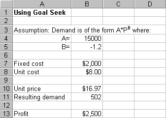
We originally entered the value $15 as the unit price in cell B10. (Any price could be entered initially.) This creates a demand of 582 and a profit of $2073. But we want the price such that profit is $2500. To find this with Goal Seek:
Use the Tools/Goal Seek menu item. In the resulting dialog box, enter B13 in the "Set cell" box, enter the value 2500 in the "To value" box, enter B10 in the "By changing cell" box, and click on OK. We see from the figure that if price is $16.97, demand will be 502, and profit will be $2500.
Goal Seek can always be used in this way. The only rules are that (1) a formula must be in the Set cell, (2) a number must be entered in the To value box, and (3) a value (not a formula) must be in the changing cell.
Using Excel's Tools/Options Menu Item
If you want to change any of Excel's default settings, the chances are that you will do so through the Tools/Options menu item. When you select this menu item, you'll see a dialog box with eight tabs at the top. (The tabs were slightly different in versions of Excel prior to Excel 97.) Each tab allows you to change a variety of settings. Although you can experiment with these, some of our favorites are the following.
![]() The View tab allows you to display or
not display a number of standard items in Excel. For example, you can uncheck
the Gridlines box if you don't want gridlines to show on a particular sheet. Or
you can uncheck the Status bar box if you want to free up more screen space for
your spreadsheet.
The View tab allows you to display or
not display a number of standard items in Excel. For example, you can uncheck
the Gridlines box if you don't want gridlines to show on a particular sheet. Or
you can uncheck the Status bar box if you want to free up more screen space for
your spreadsheet.
![]() The Calculation tab is useful for
changing the calculation mode from the default, Automatic, to one of the other
two possibilities, Automatic except tables or Manual. We especially recommend
the Automatic except tables option when replicating simulations with data
tables (as discussed in Chapter 16).
The Calculation tab is useful for
changing the calculation mode from the default, Automatic, to one of the other
two possibilities, Automatic except tables or Manual. We especially recommend
the Automatic except tables option when replicating simulations with data
tables (as discussed in Chapter 16).
![]() The General tab allows you to select
the number of sheets you want in a new workbook. The default is 3, but do you
always need 3 sheets? Remember that extra, unused sheets take up room on your
hard drive. We changed our setting to 1. In the General tab you can also change
the default file location to a directory where you store most of your files.
The General tab allows you to select
the number of sheets you want in a new workbook. The default is 3, but do you
always need 3 sheets? Remember that extra, unused sheets take up room on your
hard drive. We changed our setting to 1. In the General tab you can also change
the default file location to a directory where you store most of your files.
![]() The Custom lists tab enables you to
create your own lists for sorting. By default, sorting is done in alphabetical
order, but you can enter your own favorite list (such as Morning, Afternoon,
Evening) in the order you like. Then at a later time, when you want to sort
some data, you can ask to sort in this order. (To do so, just click on the
Options box after you use the Data/Sort menu item.)
The Custom lists tab enables you to
create your own lists for sorting. By default, sorting is done in alphabetical
order, but you can enter your own favorite list (such as Morning, Afternoon,
Evening) in the order you like. Then at a later time, when you want to sort
some data, you can ask to sort in this order. (To do so, just click on the
Options box after you use the Data/Sort menu item.)
Toolbars
It is probably easier than you think to customize toolbars. The typical setup has two toolbars at the top of the screen. These are called the Standard and Formatting toolbars. However, there are a number of other toolbars ready and waiting to be used. To see a list of them, use the Tools/Customize menu item and click on the Toolbars tab. (To see a list even quicker, right click on any toolbar that is visible.) You can check or uncheck any toolbar on the list to make it visible or invisible.
But you can do much more than this. If you select the Tools/Customize menu item and click on the Commands tab, you'll see a list of toolbar items, arranged by category. Some of these are the ones you are familiar with, while others are probably unfamiliar. Each of these items is programmed to perform some task. (Click on any item and then on the Description button to see what the item does.) If you think some of these items are more useful than the ones currently on your toolbars, just drag the old ones off and drag the new ones on. It's that easy to customize your toolbars.
If you feel adventuresome, you can even create your own toolbars and populate them with any toolbar items you like. Again, use the Tools/Customize menu item, click on the Toolbars tab, click on the New button, and enter a descriptive name. Then use the procedure in the previous paragraph to drag your favorite toolbar items to the new toolbar.