This Web site provides an active various solution algorithms for linear programming by constructing initial tableaux that are close to the optimal solution, and to improve the existing pivoting selection strategies efficiently.
To search the site, try Edit | Find in page [Ctrl + f]. Enter a word or phrase in the dialogue box, e.g. "parameter " or "linear " If the first appearance of the word/phrase is not what you are looking for, try Find Next.
MENU
- Computational Algebra Tools for Analysis of Linear Programs:
Tight Bounds for the Objective Function- Introduction
- The Ordinary Algebraic Method
- Finding all Basic Feasible Solutions
- The Refined Algebraic Method
- Numerical Examples
- Computation of Dual Prices
- Construction of the Largest Sensitivity Regions
- Construction of Simplex Final Tableau
- Concluding Remarks
- Further Readings
- An Interior Pivotal Solution Algorithm
- Which Solution Algorithm Is the Best?
- Goal-Seeking Problems
- How to Solve ILP by LP Solvers? The Cutting Plane Method
Companion Sites:
- Linear Optimization Solvers to Download
- Success Science
- Leadership Decision Making
- Linear Programming (LP) and Goal-Seeking Strategy
- Integer Optimization and the Network Models
- Tools for LP Modeling Validation
- The Classical Simplex Method
- Zero-Sum Games with Applications
- Computer-assisted Learning Concepts and Techniques
- Linear Algebra and LP Connections
- From Linear to Nonlinear Optimization with Business Applications
- Construction of the Sensitivity Region for LP Models
- Zero Sagas in Four Dimensions
- Probabilistic Modeling
- Systems Simulation
- Business Keywords and Phrases
- Collection of JavaScript E-labs Learning Objects
- Compendium of Web Site Review
- Decision Science Resources
Introduction
The Algebraic Method presented earlier, has a major deficiency in that it results in all corner points including the infeasible one which must be discarded. The simplex method is an efficient implementation of the algebraic method. However, the best known complexity result belongs to the primal dual path-following infeasible interior point methods with an iteration count of O(sqrt(n)L) to obtain an approximate solution from which the true solution can be obtained directly. Here L is the so called information length (binary coding length of input). However, the implementation of various interior point methods requires an stating point, and it has been shown that the performances of these algorithms are, unfortunately, tremendously influenced by the starting point. That is way, the simplex method still is the best algorithm that also provides useful post-optimal information for the decision makers.
The two popular approaches being taught are the primal simplex method (PS) and the dual simplex method (DS). In the PS, the initial tableau has a complete basic variable set and a non-negative RHS column. This method strives to make the last row non-positive at which point the final tableau has been achieved. In the DS, the basic variable set is also complete in the initial tableau, the last row is non-positive, and the method strives to makes the RHS non- negative.
A lot of research has been done to find a faster (polynomial) algorithm that can solve LP problems. The main branch of this research has been devoted to Interior Point Methods (IPM). The IPM outperforms the Simplex method in large LPs. However, there is still much research being done in order to improve pivoting algorithms. This Web site presents new approaches to the problem of improving the pivoting algorithms: instead of starting the Simplex with the canonical basis, we suggest as initial basis a vertex of the feasible region that is much closer to the optimal vertex than the initial solution adopted by the Simplex. By supplying the Simplex with a better initial basis, one might improve the iteration number efficiency with considerable saving in both the CPU and storage requirements.
The PS may require the use of artificial variables while the DS may require artificial constraint. These two methods are traditionally discussed in classrooms and are described more fully in traditional LP textbooks. What is novel in the artificial-free approaches is that the only requirement for the initial tableau is that the RHS is non- negative.
When one tries to solve any given problem by any of several standard phase I approaches, one becomes quickly convinced of the simplicity of the artificial-free method. Moreover, there is adequate testimony from many instructors as to the ease of insights of the concept of artificial variables or artificial constraints or artificial objective functions for business and industrial students with limited mathematical background. Precisely because these mechanisms are artificial, they lack relevance to the underlying real-world LP problem.
We present three different solution algorithms to solve any type of LP problems. All techniques are based on some extensions of the algebraic method. Before you start, put the linear program into standard form. This means making the linear program the maximization, with RHS non-negative, and changing inequality constraints (except the non-negativity conditions) to equality constraints by introducing slack/surplus variables.
The first two solution algorithms start with has no basic variables in the initial tableau. Therefore, these approaches may well provoke uneasiness and indeed disbelief among those practitioners schooled in the traditional methods which defines a simplex tableau as having a complete basic variable set. It is in this difference that the artificial-free offers a contribution to the literature.
All variables must be non-negative: Convert any unrestricted variable Xj to two non-negative variable by substituting y - Xj for every Xj everywhere. This increase the dimensionality of the problem by one only (introduce one y variable) irrespective of how many variables are unrestricted. If there are any equality constraints, one may eliminate the unrestricted variable(s) by using these equality constraints. This reduces dimensionality in both number of constraints as well as number of variables. If there is no unrestricted variables do not remove the equality constraints by substitution, this may create infeasibility. If any Xj variable is restricted to be non-positive, substitute - Xj for Xj everywhere.
The following sites enable you to practice the LP pivoting without having to do the arithmetic!
The Pivot Tool ,
tutOR, The Simplex Place, Simplex Machine, and LP-Explorer.
Further Readings:
Roos C., T. Terlaky, and J. Vial, Theory and Algorithms for Linear Optimization: An Interior Point Approach, Wiley, UK, 1997.
Junior H., and Lins, An improved initial basis for the simplex algorithm, Computers & Operations Research, 32(8), 1983-1993, 2005.
Maros I., Computational Techniques of the Simplex Method, Kluwer Publishers, 2002.
Initialization of the Simplex Method
The main idea in this solution algorithm is that the basic variable set (BVS) does not start out complete in the initial tableau, rather variables are brought in based on their contribution to the objective function value.To start the algorithm the LP problem must be converted into the following standard form:
- Must be a maximization problem,
- RHS must be non-negative,
- All variables must be non-negative,
- Convert all inequality constraints (except the non-negativity conditions) into equalities by introducing slack/surplus variables.
Step 1. Construct the initial tableau which is always considered to have empty BVS (do not occupy any row with any variable including slack variables).
BVSet Augmentation Phase:
General Strategy: Push toward optimal solution (if it exists) while maintaining feasibility. The problem is infeasible if the push towards all directions are infeasible.
Step 2. Is the BVS complete? If yes Go To Phase 2, Otherwise continue
Step 3. Pivot Column: A candidate to enter into the BVS is a non-basic variable with largest Cj (could be negative). If there are ties choose the first one from the left side. Continue
Step 4. Compute C/R (i.e. RHS/PC), Does the smallest non-negative C/R belong to an unoccupied row? If yes
Pivot Row: Enter the variable into BVS by performing the GJ row operations, and return to Step 2. If Not Go To Step 5
Step 5. Is there any other non-basic variable as candidate to enter? If yes the next variable with the largest Cj and Go to Step 4. Otherwise go to previous tableaux and try other possibilities. If all possibilities are exhausted then the problem is infeasible.
Optimality (Simplex) Phase:
General Strategy: Move from corner point to a better corner point in the search of optimal corner point (or the problem is unbounded).
Step 6. Are all Cj non-positive in the current tableau? If yes, go to Step 8; Otherwise continue.
Step 7. Apply the (ordinary) simplex method rules for entering and exiting variables to and from BVS). Go to 6.
Step 8. This is an optimal tableau. Find out all multiple solutions (if the number of Cj = 0 is larger than the size of the BVS) if they exist.
Notes: We make no claim as to computational performance. Nor do we have a pretense that our method always permits solutions in m (the number of constraints) iterations without trying all other possibilities before declaring infeasibility. An algorithm with such performance would indeed be remarkable. At this time the intent is solely to provide an efficient and effective tool for students to do LP by hand-computation without cumbersome inventions
Numerical Examples
The following sites enable you to practice the LP pivoting without having to do the arithmetic!
The Pivot Tool ,
tutOR, The Simplex Place, Simplex Machine, and LP-Explorer.
Example 1: The following problem is attributed to Gert Tijssen.
Max -X1 - 4X2 - 2X3,
subject to:
X1 - X2 + X3 = 0,
-X2 + 4X3 = 1,
and X1, X2, X3 ³ 0.
Since the constraints are already in equality form, the initial tableau is readily available for this problem:
| BVS | X1 | X2 | X3 | RHS | C/R | |
|---|---|---|---|---|---|---|
| ? | (1) | -1 | 1 | 0 | 0/1 | |
| ? | 0 | -1 | 4 | 1 | -- | |
| Cj | -1 | -4 | -2 |
By Step 3, the candidate variable to enter is X1 and by Step 4 the smallest C/R belongs to an open row, so its position is the first row. After pivoting we get:
| BVS | X1 | X2 | X3 | RHS | C/R | |
|---|---|---|---|---|---|---|
| X1 | 1 | -1 | 1 | 0 | -- | |
| ? | 0 | -1 | 4 | 1 | 1/4 | |
| Cj | 0 | -5 | -1 |
The next candidate variable to enter is X3, performing GJ pivoting the RHS(1) becomes negative. Therefore, we should try X2. The C/R is negative. As indicated in Step 5, we go back to step 2 to try other candidates.
Consider the previous tableau; instead of bringing X1 in we try the next candidate, which is X3:
| BVS | X1 | X2 | X3 | RHS | C/R | |
|---|---|---|---|---|---|---|
| ? | 1 | -1 | (1) | 0 | 0/1 | |
| ? | 0 | -1 | 4 | 1 | 1/4 | |
| Cj | -1 | -4 | -2 |
Its location is the first row, after performing the GJ operations, we have:
| BVS | X1 | X2 | X3 | RHS | C/R | |
|---|---|---|---|---|---|---|
| X3 | 1 | -1 | 1 | 0 | -- | |
| ? | -4 | 3 | 0 | |||
| Cj | 1 | -6 | 0 |
The candidate variable to enter is X1, however its C/R is negative. Therefore, we pick the next candidate, which is X2. Bringing X2 into BVS, we have:
| BVS | X1 | X2 | X3 | RHS | |
|---|---|---|---|---|---|
| X3 | -1/3 | 0 | 1 | 1/3 | |
| X2 | -4/3 | 1 | 0 | 1/3 | |
| Cj | -7 | 0 | 0 |
This is the end of phase 1. The tableau is already optimal. There is no need for phase 2. The optimal solution is: X1 = 0, X2 = 1/3, X3 = 1/3, with the optimal value of -2.
Example 2: The following problem is attributed to Andreas Enge, and Peter Huhn.
Maximize 3X1 + X2 - 4X3
subject to:
X1 + X2 - X3 =1
X2 ³ 2
X1 ³ 0
X3 ³ 0
After adding a surplus variable, the initial tableau is:
| BVS | X1 | X2 | X3 | S1 | RHS | |
|---|---|---|---|---|---|---|
| ? | 1 | 1 | -1 | 0 | 1 | |
| ? | 0 | 1 | 0 | -1 | 2 | |
| Cj | 3 | 1 | -4 | 0 |
Bringing X1 into bases we have:
| BVS | X1 | X2 | X3 | S1 | RHS | |
|---|---|---|---|---|---|---|
| X1 | 1 | 1 | -1 | 0 | 1 | |
| ? | 0 | 1 | 0 | -1 | 2 | |
| Cj | 0 | -2 | -1 | 0 |
Now we cannot bring any variables in while maintaining feasibility. However before declaring infeasibility for the problem we must try other possibilities. Going back to the tableau just before the current one, we try to bring in X2:
| BVS | X1 | X2 | X3 | S1 | RHS | |
|---|---|---|---|---|---|---|
| X2 | 1 | 1 | -1 | 0 | 1 | |
| ? | -1 | 0 | 1 | -1 | 1 | |
| Cj | 2 | 0 | -3 | 0 |
X1 , and S1 cannot come in since they make some RHS values negative. The next variables to come in is X3. The next tableau is the final one.
| BVS | X1 | X2 | X3 | S1 | RHS | |
|---|---|---|---|---|---|---|
| X2 | 0 | 1 | 0 | -1 | 2 | |
| X3 | -1 | 0 | 1 | -1 | 1 | |
| Cj | -1 | 0 | 0 | -3 |
The optimal solution is X1 = 0, X2 = 2, X3 = 1, with S1= 0.
Example 3: The following problem is attributed to Richard Cottle, Jong-Shi Pang, Richard Stone of Burnsville, Minnesota, and Crnig Tovey.
Maximize 2X1 + 3X2 - 6X3
subject to:
X1 + 3X2 + 2X3 £ 3,
- 2X2 + X3 £ 1
X1 - X2 + X3 = 2
2X1 + 2X2 - 3X3 = 0
X1 , X2 , X3 ³ 0
The initial tableau is:
| BVS | X1 | X2 | X3 | S1 | S2 | RHS | |
|---|---|---|---|---|---|---|---|
| ? | 1 | 3 | 2 | 1 | 0 | 3 | |
| ? | 0 | -2 | 1 | 0 | 1 | 1 | |
| ? | 1 | -1 | 1 | 0 | 0 | 2 | |
| ? | 2 | 2 | -3 | 0 | 0 | 0 | |
| Cj | 2 | 3 | -6 | 0 | 0 |
Bringing X2 into BVS gives an infeasible sign after one iteration. Therefore we try to bring in X1:
| BVS | X1 | X2 | X3 | S1 | S2 | RHS | |
|---|---|---|---|---|---|---|---|
| ? | 0 | 2 | 7/2 | 1 | 0 | 3 | |
| ? | 0 | -2 | 1 | 0 | 1 | 1 | |
| ? | 0 | -2 | 5/2 | 0 | 0 | 2 | |
| X1 | 1 | 1 | -3/2 | 0 | 0 | 0 | |
| Cj | 0 | 1 | -3 | 0 | 0 |
X2 cannot come in since it makes some RHS negative. The next variables to come in are S1 and S2 without any GJ iterations.
| BVS | X1 | X2 | X3 | S1 | S2 | RHS | |
|---|---|---|---|---|---|---|---|
| S1 | 0 | 2 | 7/2 | 1 | 0 | 3 | |
| S2 | 0 | -2 | 1 | 0 | 1 | 1 | |
| ? | 0 | -2 | 5/2 | 0 | 0 | 2 | |
| X1 | 1 | 1 | -3/2 | 0 | 0 | 0 | |
| Cj | 0 | 1 | -3 | 0 | 0 |
Therefore we try to bring in X3. The next tableau is the final one.
| BVS | X1 | X2 | X3 | S1 | S2 | RHS | |
|---|---|---|---|---|---|---|---|
| S1 | 0 | 24/5 | 0 | 1 | 0 | 1/5 | |
| S2 | 0 | -6/5 | 0 | 0 | 1 | 1/5 | |
| X3 | 0 | -4/5 | 1 | 0 | 0 | 4/5 | |
| X1 | 1 | -1/5 | 0 | 0 | 0 | 6/5 | |
| Cj | 0 | -7/5 | 0 | 0 | 0 |
This is the end of phase 1. The tableau is already optimal. There is no need for phase 2. The optimal solution for decision variables are: X1 = 6/5, X2 = 0, X3 = 4/5.
Example 4: Consider the following problem:
Max -X1 + 2X2
subject to:
X1 + X2 ³ 2,
-X1 + X2 ³ 1,
X2 £ 3,
and X1, X2 ³ 0.
Converting the constraints into equality form, we have:
X1 + X2 - S1 = 2,
-X1 + X2 - S2 = 1,
X2 + S3 = 3
The initial tableau for this problem is:
| BVS | X1 | X2 | S1 | S2 | S3 | RHS | C/R | |
|---|---|---|---|---|---|---|---|---|
| ? | 1 | 1 | -1 | 0 | 0 | 2 | 2/1 | |
| ? | -1 | (1) | 0 | -1 | 0 | 1 | 1/1 | |
| ? | 0 | 1 | 0 | 0 | 1 | 3 | 3/1 | |
| Cj | -1 | 2 | 0 | 0 | 0 |
Although S3 could be considered as a BV, but as always we start phase 1 with an empty BVS. By Step 3 of the algorithm, the candidate variable to enter is X2 and by Step 4 the smallest C/R belongs to an open row, so its position is the second row. After pivoting we get:
| BVS | X1 | X2 | S1 | S2 | S3 | RHS | C/R | |
|---|---|---|---|---|---|---|---|---|
| ? | 2 | 0 | -1 | (1) | 0 | 1 | 1/1 | |
| X2 | -1 | 1 | 0 | -1 | 0 | 1 | -- | |
| ? | 1 | 0 | 0 | 1 | 1 | 2 | 2/1 | |
| Cj | 1 | 0 | 0 | 2 | 0 |
The next variable to enter is S2, which is the slack/surplus of an occupied row namely the second row. Performing GJ pivoting we get:
| BVS | X1 | X2 | S1 | S2 | S3 | RHS | C/R | |
|---|---|---|---|---|---|---|---|---|
| S2 | 2 | 0 | -1 | 1 | 0 | 1 | -- | |
| X2 | 1 | 1 | -1 | 0 | 0 | 2 | -- | |
| ? | -1 | 0 | (1) | 0 | 1 | 1 | 1/1 | |
| Cj | -3 | 0 | 2 | 0 | 0 |
The next incoming variable is S1, generating the next tableau, we obtain:
| BVS | X1 | X2 | S1 | S2 | S3 | RHS | C/R | |
|---|---|---|---|---|---|---|---|---|
| S2 | 1 | 0 | 0 | 1 | 1 | 2 | ||
| X2 | 0 | 1 | 0 | 0 | 1 | 3 | ||
| S1 | -1 | 0 | 1 | 0 | 1 | 1 | ||
| Cj | -1 | 0 | 0 | -2 |
This is the end of phase 1. The tableau is already optimal. There is no need for phase 2. The optimal solution for decision variables are: X1 = 0, X2 = 3 with the optimal value, which is found by plugging the optimal decision into the original objective function, we get the optimal value = 6.
Example 5: Consider the following problem:
Max 6X1 + 2X2
Subject to: 2X1 + 4X2 £ 20, 3X1 + 5X2 ³ 15, X1 ³3, X2³ 0.
The Initial tableau:
| BVS | X1 | X2 | S1 | S2 | S3 | RHS | C/R | |
|---|---|---|---|---|---|---|---|---|
| S1 | 2 | 4 | 1 | 0 | 0 | 20 | --- | |
| ? | 3 | 5 | 0 | -1 | 0 | 15 | 15/3 = 5 | |
| ? | 1 | 0 | 0 | 0 | -1 | 3 | 3/1 = 3 | |
| Cj | 6 | 2 | 0 | 0 | 0 |
X1 enters into the BVS. First tableau is:
| BVS | X1 | X2 | S1 | S2 | S3 | RHS | C/R | |
|---|---|---|---|---|---|---|---|---|
| S1 | 0 | 4 | 1 | 0 | 2 | 14 | -- | |
| ? | 0 | 5 | 0 | -1 | 3 | 6 | 6/3 = 2 | |
| X1 | 1 | 0 | 0 | 0 | -1 | 3 | -- | |
| Cj | 0 | 2 | 0 | 0 | 6 |
Now S3 enters. The second tableau is:
| BVS | X1 | X2 | S1 | S2 | S3 | RHS | C/R | |
|---|---|---|---|---|---|---|---|---|
| S1 | 0 | 2/3 | 1 | 2/3 | 0 | 10 | 10/(2/3) =15 | |
| S3 | 0 | 5/3 | 0 | -1/3 | 1 | 2 | -- | |
| X1 | 1 | 5/3 | 0 | -1/3 | 0 | 5 | -- | |
| Cj | 0 | -8 | 0 | 2 | 0 |
The BVS is complete. Start the ordinary Simplex method.
| BVS | X1 | X2 | S1 | S2 | S3 | RHS | |
|---|---|---|---|---|---|---|---|
| S2 | 0 | 1 | 3/2 | 1 | 0 | 15 | |
| S3 | 0 | 2 | 1/2 | 0 | 1 | 7 | |
| X1 | 1 | 2 | 1/2 | 0 | 0 | 10 | |
| Cj | 0 | -10 | -3 | 0 | 0 |
This is the final tableau, which provides all the following information. The optimal solution is X = 10, X = 0. The slack and surpluses are S = 0, S = 15, S = 7. The solution to the dual problems are: U = 3, U = 0, and U = 0.
Example 6: Solve the following problem:
Consider the following problem:
Max 3X1 + 5X2,
subject to:
2X1 + X2 = 10,
X1, and X2 ³ 0.
Since the constraint is already in equality form, the initial tableau is readily available for this problem:
| BVS | X1 | X2 | RHS | |
|---|---|---|---|---|
| ? | 2 | (1) | 10 | |
| Cj | 3 | 5 |
By Step 3, the candidate variable to enter is X2 and there is only one open row, so its position is the first row. After pivoting we get:
| BVS | X1 | X2 | RHS | |
|---|---|---|---|---|
| X2 | 2 | 1 | 10 | |
| Cj | -7 | 0 |
This is the end of phase 1. The tableau is already optimal. There is no need for phase 2. The optimal solution is: X1 = 0, X2 = 10, with the optimal value of 50.
Now the question is: How to compute the shadow price? The dual problem is
Min 10U1
subject to:
2U1 £ 3,
U1 £ 5,
and U1 is unrestricted in sign.
Since X2 in not zero, the second constraint in the dual problem must be binding (by the complementary slackness theorem). This gives the solution to the dual problem as U1 = 5, with the same optimal value = 50 as expected. Therefore, the shadow price for the RHS of the primal problem is equal to 5.
Example 7: By default, in this solution algorithm just like almost all LP solvers (such as LINDO), we assumed that all variables are non-negative.
To achieve this requirement, convert any unrestricted variable Xj to two non-negative variable by substituting y - Xj for every Xj everywhere. This increases the dimensionality of the problem by one only (introduce one y variable) irrespective of how many variables are unrestricted.
If any Xj variable is restricted to be non-positive, substitute - Xj for Xj everywhere. This reduces the complexity of the problem.
Solve the converted problem, and then substitute back to get the values for the original variables.
The following numerical example illustrates the process:
Maximize -X1
subject to:
X1 + X2 ³ 0,
X1 + 3X2 £ 3.
The converted problem is:
Maximize -y + X1
subject to:
-X1 - X2 + 2y ³ 0,
-X1 - 3X2 + 4y £ 3,
X1 ³ 0,
X2 ³ 0,
and y ³ 0.
| BVS | X1 | X2 | y | S1 | S2 | RHS | C/R | |
|---|---|---|---|---|---|---|---|---|
| ? | -1 | -1 | 2 | -1 | 0 | 0 | 0/2 | |
| ? | -1 | -3 | 4 | 0 | 1 | 3 | 3/3 | |
| Cj | 1 | 0 | -1 | 0 | 0 |
The first variable to come in is X1:
| BVS | X1 | X2 | y | S1 | S2 | RHS | C/R | |
|---|---|---|---|---|---|---|---|---|
| X1 | 1 | 1 | -2 | 1 | 0 | 0 | -- | |
| ? | 0 | -2 | 2 | 1 | 1 | 3 | 3/2 | |
| Cj | 0 | -1 | 1 | -1 | 0 |
The next variable to come in is y:
| BVS | X1 | X2 | y | S1 | S2 | RHS | |
|---|---|---|---|---|---|---|---|
| X1 | 1 | -1 | 0 | 2 | 1 | 3 | |
| y | 0 | -1 | 1 | 1/2 | 1/2 | 3/2 | |
| Cj | 0 | 0 | 0 | -3/2 | -1/2 |
The optimal solution for the original variables is: X1 = 3/2 - 3 = -3/2, X2 = 3/2 - 0 = 3/2, with optimal value of 3/2.
Is there any other optimal solutions? Notice that the number of zeros in the last row of the final tableau exceeds the number of basic variables (this is the necessary condition for the existence of multiple solutions), however, one cannot bring in X2 into the basic variable set. Therefore, this solution is the only optimal solution.
Further Readings:
Arsham H., Initialization of the simplex algorithm: An artificial-free approach, SIAM Review, Vol. 39, No. 4, 736-744, 1997.
Arsham H., An artificial-free simplex algorithm for general LP models, Mathematical and Computer Modelling, Vol. 25, No. 1, 107-123, 1997.
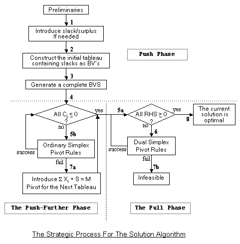
The Push-and-Pull Solution Algorithm
The initial tableau may be empty, partially empty, or contain a full basic variable set (BVS). The proposed scheme consists of the following three strategic phases:
Push Fill-up the BVS completely by pushing it toward the optimal corner point, while trying to maintain feasibility.
Push Further If the BVS is complete, but the optimality condition is not satisfied, then push further until this condition is satisfied.
Pull If pushed too far in Phase I, pull back toward the optimal corner point (if any). If the BVS is complete, and the optimality condition is satisfied but infeasible, then pull back to the optimal corner point; i.e., a dual simplex approach.
Not all LP problems must go through the Push, Push Further and Pull sequence of steps, as shown in the numerical examples.
To start the algorithm the LP problem must be converted into the following standard form:
- Must be a maximization problem
- RHS must be non-negative
- All variables must be non-negative
- Convert all inequality constraints (except the non-negativity conditions) into equalities by introducing slack/surplus variables.
The following three phases describe how the algorithm works. It terminates successfully for any type of LP problems since there is no loop-back between the phases.
Step 1. By introducing slack or surplus variables convert all inequalities (except non-negativity) constraints into equalities. The coefficient matrix must have full row rank, since otherwise either no solution exists or there are redundant equations.
Step 2. Construct the initial tableau containing all slack variables as basic variables.
Step 3. Generate a basic variable (BV) set, not necessarily feasible, as follow:
- Incoming variable is Xj with the largest Cj (the coefficient of Xj in the objective function, it could be negative), and if possible with smallest non-negative C/R. Otherwise try the next variable to enter. If there are alternatives, break the ties arbitrarily.
- Is Xj the last variable to enter into BV set? If yes, enter it into the empty row and generate the next tableau (if impossible to pivot, go to Step 3(1) and choose the next Cj) and go to Step 4. Otherwise its row position is the row having the smallest non-negative C/R. Do not consider the rows, which are already occupied. If there are alternative, break the ties arbitrarily.
Generate the next tableau and go to Step 3(1). If there is no positive C/R, then select the row having smallest non-negative C/R.
Step 4. Are all Cj £ 0 in the current tableau? If yes, go to Step 5a; otherwise go to Step 5b.
Step 5a. Are all RHS ³ 0 in the current tableau? If yes, go to Step 8. Otherwise go to Step 6.
Step 5b. Use the ordinary simplex pivoting rule:
- Identify incoming variable (having largest Cj).
- Identify outgoing variable (with the smallest non-negative C/R). If none, unbounded solution. (If more than one choose any one, this may be the sign of degeneracy.) Generate the next tableau and go to Step 4. If Step 5b fails, then go to step 7a.
Step 7a If all RHS ³ 0 , then the optimal solution is unbounded. Otherwise , introduce a new constraint SXi + S = M to the current tableau, with S as a basic variable. Where M is an unspecified sufficiently, large positive number, and Xi's are variables with a positive Cj in the current tableau. Enter the variable with largest Cj and exit S. Generate the next tableau, (this makes all Cj £ 0), then go to Step 5a.
Step 6. Use the dual simplex pivoting rules to identify the outgoing variable (smallest RHS). Identify the incoming variable having negative coefficient in the pivot row in the current tableau, if there are alternatives choose the one with the smallest positive row ratio (R/R), [that is, a new row with elements: row Cj/pivot row]; if otherwise generate the next tableau and to Step 5a. If Step 6 fails, then go to Step 7b.
Step 7b. The problem is infeasible. Stop.
Step 8. This is the optimal solution, which could be unbounded. Find out all multiple solutions if they exist (the if the number of Cj = 0 is larger than the size of the BV set, this is a necessary condition).
The algorithmic strategic process is presented in the following flowchart.
Notes:
1. By following Steps 3(1) and 3(2) a complete BV set can always be generated, which may not be feasible. Proof of the first part of this statement follows by contradiction (from the fact that there is no redundancy/inconsistency among the constraints). The second part indicates that by pushing toward the optimal corner point we may have passed it.
2. Note that if all elements in any row are zero, we have one of two special cases. If the RHS element is non-zero then the problem is infeasible. If the RHS is zero this row represents a redundant constraint. Delete this row and proceed.
3. If you ever reach to the Step 7a or 7b, you must go back and check the formulation of the problem, since the problem could be unbounded.
Numerical Examples:
The following sites enable you to practice the LP pivoting without having to do the arithmetic!
The Pivot Tool ,
tutOR, The Simplex Place, Simplex Machine, and LP-Explorer .
Example 1: The following problem is attributed to Gert Tijssen.
Max -X1 - 4X2 - 2X3,
subject to:
X1 - X2 + X3 = 0,
-X2 + 4X3 = 1,
and X1, X2, X3 ³ 0.
Since the constraints are already in equality form, the initial tableau is readily available for this problem:
| BVS | X1 | X2 | X3 | RHS | C/R | |
|---|---|---|---|---|---|---|
| ? | (1) | -1 | 1 | 0 | 0/1 | |
| ? | 0 | -1 | 4 | 1 | -- | |
| Cj | -1 | -4 | -2 |
The Push Phase: The candidate variable to enter is X1 and the smallest C/R belongs to an open row, so its position is the first row. After pivoting we get:
| BVS | X1 | X2 | X3 | RHS | C/R | |
|---|---|---|---|---|---|---|
| X1 | 1 | -1 | 1 | 0 | -- | |
| ? | 0 | -1 | (4) | 1 | 1/4 | |
| Cj | 0 | -5 | -1 |
The next candidate variable to enter is X3, performing GJ we have:
| BVS | X1 | X2 | X3 | RHS | |
|---|---|---|---|---|---|
| X1 | 1 | -3/4 | 0 | -1/4 | |
| X3 | 0 | -1/4 | 1 | 1/4 | |
| Cj | 0 | -21/4 | 0 | ||
| R/R | - | 21/3 | - |
Push Further Phase: There is no need for this phase since all Cj's are non-positive.
The Pull Phase: The variable to go out is X1. By row-ratio criterion, the variable to come is X2. After performing the GJ operations, we have:
| BVS | X1 | X2 | X3 | RHS | |
|---|---|---|---|---|---|
| X2 | -1/3 | 0 | 1 | 1/3 | |
| X3 | -4/3 | 1 | 0 | 1/3 | |
| Cj | -7 | 0 | 0 |
This tableau is the optimal one. The optimal solution is : X1 = 0, X2 = 1/3, X3 = 1/3. With the optimal value, which is found by plugging the optimal decision into the original objective function, we get the optimal value = -2.
Example 2: The following problem is attributed to Andreas Enge, and Peter Huhn.
Maximize 3X1 + X2 - 4X3
subject to:
X1 + X2 - X3 =1
X2 ³ 2
X1 ³ 0
X3 ³ 0
After adding a surplus variable, the initial tableau is:
| BVS | X1 | X2 | X3 | S1 | RHS | |
|---|---|---|---|---|---|---|
| ? | 1 | 1 | -1 | 0 | 1 | |
| ? | 0 | 1 | 0 | -1 | 2 | |
| Cj | 3 | 1 | -4 | 0 |
The Push Phase: Bringing X1 into bases we have:
| BVS | X1 | X2 | X3 | S1 | RHS | |
|---|---|---|---|---|---|---|
| X1 | 1 | 1 | -1 | 0 | 1 | |
| ? | 0 | 1 | 0 | -1 | 2 | |
| Cj | 0 | -2 | -1 | 0 |
Now bring S1 into BVS:
| BVS | X1 | X2 | X3 | S1 | RHS | |
|---|---|---|---|---|---|---|
| X1 | 1 | 1 | -1 | 0 | 1 | |
| S1 | 0 | -1 | 0 | 1 | -2 | |
| Cj | 0 | -2 | -1 | 0 | ||
| R/R | -- | 2 | -- | -- |
Push Further Phase: There is no need for this phase since all Cj's are non-positive.
The Pull Phase: S1 goes out and X3 comes in:
| BVS | X1 | X2 | X3 | S1 | RHS | |
|---|---|---|---|---|---|---|
| X1 | 1 | 0 | -1 | 1 | -1 | |
| X2 | 0 | 1 | 0 | -1 | 2 | |
| Cj | 0 | 0 | -1 | -2 | ||
| R/R | -- | -- | 1 | 2 |
The Pull Phase: X1 goes out and X3 comes in.
| BVS | X1 | X2 | X3 | S1 | RHS | |
|---|---|---|---|---|---|---|
| X3 | -1 | 0 | 1 | -1 | 1 | |
| X2 | 0 | 1 | 0 | -1 | 2 | |
| Cj | -1 | 0 | 0 | -3 |
This tableau is optimal. The optimal solution is X1 = 0, X2 = 2, X3 = 1, with S1= 0.
Example 3: The following problem is attributed to Richard Cottle, Jong-Shi Pang, Richard Stone, and Crnig Tovey.
Maximize 2X1 + 3X2 - 6X3
subject to:
X1 + 3X2 + 2X3 £ 3,
- 2X2 + X3 £ 1
X1 - X2 + X3 = 2
2X1 + 2X2 - 3X3 = 0
X1 , X2 , X3 ³ 0
The initial tableau is:
| BVS | X1 | X2 | X3 | S1 | S2 | RHS | |
|---|---|---|---|---|---|---|---|
| S1 | 1 | 3 | 2 | 1 | 0 | 3 | |
| S2 | 0 | -2 | 1 | 0 | 1 | 1 | |
| ? | 1 | -1 | 1 | 0 | 0 | 2 | |
| ? | 2 | (2) | -3 | 0 | 0 | 0 | |
| Cj | 2 | 3 | -6 | 0 | 0 |
The Push Phase: Bringing X2 into BVS gives the following tableau:
| BVS | X1 | X2 | X3 | S1 | S2 | RHS | |
|---|---|---|---|---|---|---|---|
| S1 | -2 | 0 | 13/2 | 1 | 0 | 3 | |
| S2 | 2 | 0 | -2 | 0 | 1 | 1 | |
| ? | 2 | 0 | -1/2 | 0 | 0 | 2 | |
| X2 | 1 | 1 | -3/2 | 0 | 0 | 0 | |
| Cj | -1 | 0 | -3/2 | 0 | 0 |
The next variable is X1 to come in:
| BVS | X1 | X2 | X3 | S1 | S2 | RHS | |
|---|---|---|---|---|---|---|---|
| S1 | 0 | 0 | 6 | 1 | 0 | 5 | |
| S2 | 0 | 0 | -3/2 | 0 | 1 | -1 | |
| X1 | 1 | 0 | -1/4 | 0 | 0 | 1 | |
| X2 | 0 | 1 | (-5/4) | 0 | 0 | -1 | |
| Cj | 0 | 0 | -7/4 | 0 | 0 | ||
| R/R | -- | -- | 7/5 | -- | -- |
Push Further Phase: There is no need for this phase since all Cj's are non-positive.
The Pull Phase: The variable to go out is X2. By row ratio, X3 comes in
| BVS | X1 | X2 | X3 | S1 | S2 | RHS | |
|---|---|---|---|---|---|---|---|
| S1 | 0 | 24/5 | 0 | 1 | 0 | 1/5 | |
| S2 | 0 | -6/5 | 0 | 0 | 1 | 1/5 | |
| X1 | 1 | -1/5 | 0 | 0 | 0 | 6/5 | |
| X3 | 0 | -4/5 | 1 | 0 | 0 | 4/5 | |
| Cj | 0 | -7/5 | 0 | 0 | 0 |
This tableau is the optimal one. The optimal solution for decision variables are: X1 = 6/5, X2 = 0, and X3 = 4/5.
Computer Implementation and comparison with other algorithms: For the computerized implementation of this algorithm, some refinements might be needed. For example, in deciding on exchanging the variables, one might consider to total contribution, rather than marginal contribution to the current objective function value. In other words, recall that the choice of smallest non-negative C/R provide the marginal change in the objective function, while maintaining feasibility. However, since we are constructing the C/R for all candidate variables, we may obtain the largest contribution by considering the product Cj (C/R) in our selection rule. The following example illustrates this enhancement in the algorithm:
Example 4: The following problem is attributed to Klee and Minty.
Max 100X1 + 10X2 + X3,
subject to:
X1 £ 1,
20X1 + X2 £ 100,
200X1 + 20X2 + X3 £ 100000,
and X1, X2, X3 ³ 0.
This example is constructed to show that the Simplex method is exponential in its computational complexity. For this example with n= 3, it takes 23 = 8 iterations.
Converting the constraints to equalities, we have:
Max 100X1 + 10X2 + X3,
subject to:
X1 + S1 = 1,
20X1 + X2 + S2 = 100,
200X1 + 20X2 + X3 + S3 = 100000,
and X1, X2, X3 ³ 0.
Phase 1: The initial tableau with the two slack variables as its BV is:
| BVS | X1 | X2 | X3 | S1 | S2 | S3 | RHS | C/R1 | C/R2 | C/R3 | ||||
|---|---|---|---|---|---|---|---|---|---|---|---|---|---|---|
| S1 | 1 | 0 | 0 | 1 | 0 | 0 | 1 | 1 | -- | -- | ||||
| S2 | 20 | 1 | 0 | 0 | 1 | 0 | 100 | 5 | 100 | -- | ||||
| S3 | 200 | 20 | 1 | 0 | 0 | 1 | 100000 | 500 | 5000 | 100000 | ||||
| Cj | 100 | 10 | 1 | 0 | 0 | 0 |
Total Contribution Criterion:
- The smallest non-negative C/R1 is 1, which belongs to X1, with marginal contribution of C1 = 100. Therefore, its total contribution to the current objective function value is C1(C/R1)= 100(1) = 100.
- The smallest non-negative C/R2 is 100, which belongs to X2, with marginal contribution of C2 = 10. Therefore, its total contribution to the current objective function value is C2(C/R2)= 10(100) = 1000.
- The smallest non-negative C/R3 is 100000, which belongs to X3 with marginal contribution of C3 = 1. Therefore, its total contribution to the current objective function value is C3(C/R3)= 1(100000) = 100000.
The Push Further Phase: The candidate variables to enter are X1, X2, and X3 with C/R shown in the above table. Based on the total contribution criterion, the largest contribution to the objective function achieved by bringing X3 in. Therefore, replacing S3 with X3, after pivoting we get:
| BVS | X1 | X2 | X3 | S1 | S2 | S3 | RHS | |
|---|---|---|---|---|---|---|---|---|
| S1 | 1 | 0 | 0 | 1 | 0 | 0 | 1 | |
| S2 | 20 | 1 | 0 | 0 | 1 | 0 | 100 | |
| X3 | 200 | 20 | 1 | 0 | 0 | 1 | 100000 | |
| Cj | -100 | -10 | 0 | 0 | 0 | -1 |
This tableau is the optimal one. The optimal solution is: X1 = 100000, X2 = 0, X3 = 0, with the optimal value of 100000.
You may like to install LP Solvers software package on your computer, and checking your computations or for solving larger problems.
Further Readings: Arsham H., et al., A computer implementation of the push-and-pull algorithm and its computational comparison with LP simplex method, Applied Mathematics and Computation, Vol. 170, No. 1, 36-63, 2005.
Arsham H., et al., An algorithm for simplex tableau reduction: The push-and-pull solution strategy, Applied Mathematics and Computation, Vol. 137, No. (2-3), 525-547, 2003.
Arsham H., et al., An algorithm for simplex tableau reduction with numerical comparisons, International Journal of Pure and Applied Mathematics, Vol. 4, No. 1, 57-85, 2003.
Arsham H., A tabular, simplex type algorithm as a teaching aid for general LP models, Mathematical and Computer Modelling, Vol. 12, No. 8, 1051-1056, 1989.
Klee V., and G. Minty, How good is the simplex algorithm, in Inequalities-III, Edited by O. Shisha, Academic Press, 1972, 159-175.
Greater-than-or-equal Constraints Relaxation Method
We start with an LP problem in the following standard form:
Max Z = C . X
subject to
AX £ a
BX ³ b
all X ³ 0,
where b ³ 0, a > 0
Note that the main constraints have separated into two subgroups. A and B are the respective matrices of constraint coefficients, and a and b are the respective RHS vectors (all with appropriate dimensions). Without loss of generality we assume all the RHS elements are non-negative. We will not deal with the trivial cases such as when A=B=0, (no constraints) or a=b=0 (all boundaries pass through the origin). The customary notation is used: Z for the objective, Cj for the cost coefficients, and X for the decision vector. Here, the word constraints means any constraint other than the nonnegativitiy conditions. In this standard form, whenever the RHS is zero, this constraint should be considered as since b is allowed to be 0 but a is not. We depart from the usual convention by separating the constraints into two groups according to £ and ³.
To arrive at this form any general problem some of the following preliminaries may be necessary.
- Convert unrestricted variables (if any) to non-negative.
- Make all RHS non-negative.
- Convert equality constraints (if any) into a pair of ³ and £ constraints.
- Remove £ constraints for, which all coefficients are non-positive. This eliminates constraints, which are redundant with the first quadrant constraint.
- The existence of any ³ constraints for, which all coefficients are non- positive and RHS positive, indicates that the problem is infeasible.
- Convert all £ inequality constraints with RHS = 0 into ³ 0. This may avoid degeneracy at the origin.
The following provides an overview of the algorithm's strategy considering the most interesting common case, (a mixture of ³ and £ constraints). This establishes a framework to, which we then extend to complete generality. We proceed as follows:
Phase 1: Relax the ³ constraints and solve the reduced problem with the usual simplex. In most cases we obtain an optimal simplex tableau, i.e. a tableau, which satisfies both optimality and feasibility conditions.
(The discussion of several special cases is deferred for the moment.)
Phase 2: If the solution satisfies all the relaxed constraints, we are done. Otherwise we bring the most "violated" constraint into the tableau and use dual simplex to restore feasibility. This process is repeated until all constraints are satisfied. This step involves several special cases to be discussed after the primary case.
Phase 3: Restore the original objective function (if needed) as follows. Replace the last row in the current tableau to its original values and catch up. Perform the usual simplex. If this is not successful, the problem is unbounded; otherwise the current tableau contains the optimal solution. Extract the optimal solution and multiple solutions (if any).
Special Cases: Three special cases arise in Phase 1, which may require special treatment. If all constraints are ³ and the objective function coefficients satisfy the optimality condition, the origin satisfies the optimality condition but is infeasible. Relax all constraints and start with origin. Some cases may not prove optimal (the relaxed problem has an unbounded feasible region). In Phase 1. the current objective function is changed in a prescribed manner. If all constraints are ³, the origin is not feasible, and if there is any positive Cj we have to change it to 0. This requires restoration of the original objective function, which is done in Phase 3.
Notice that unlike simplex and dual simplex, we focus on the most active constraints rather than carrying all constraints in the initial and all subsequent tableaux. We bring ³ constraints one by one into our tables. This may also reduce computational effort.
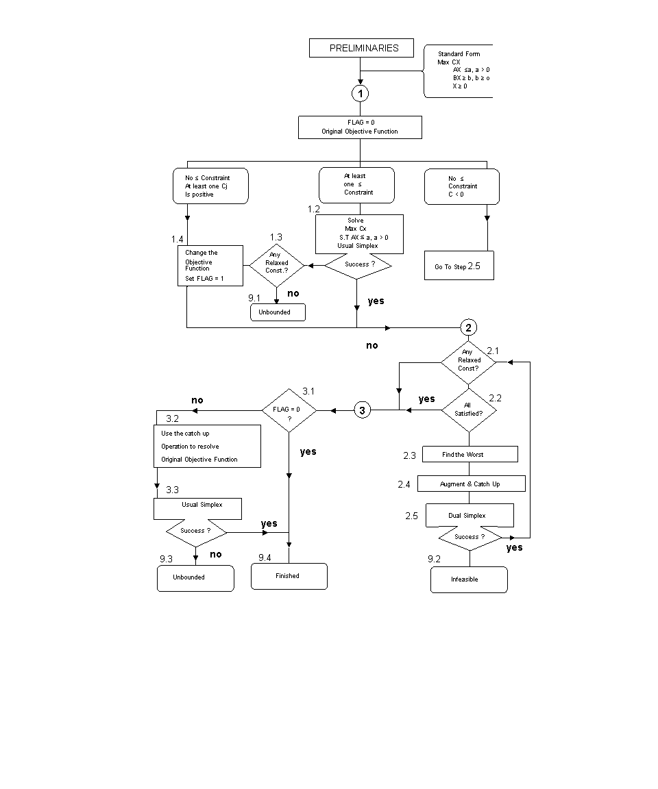
Greater-than-or-equal Constraints Relaxation Method
Click on the image to enlarge it
Detailed Process:
PHASE 1: Recognize three cases as follows:
Step 1.1 Set FLAG=0. This indicates the original objective function is still in use. Check the existence of £ constraints and the signs of the Cjs.
Distinguish there, three possibilities:
a) There is at least one £ constraint. Go to Step 1.2.
b) There are no £ constraints, and no Cj is positive. The origin is the current solution. Go to PHASE 2.
c) There are no £ constraints, and at least one Cj is positive (i.e. A = 0, Cj > 0 at least for one j). Go to Step 1.4.
Step 1.2 From the standard problem relax temporarily all ³ constraints with positive RHS. Solve the sub-problem using the usual Simplex. If successful go to PHASE 2.
Otherwise, go to Step 1.3.
Step 1.3 Are there any ³ constraints?
If yes, go to Step 1.4.
Otherwise go to Step 9.1.
Step 1.4 Change all Cj > 0 elements to 0. Set the FLAG=1. The origin is the starting point. Go to PHASE 2.
Step 9.1 The original problem is unbounded.
PHASE 2: Bring in relaxed constraints (if needed) as follows:
Step 2.1 If there are any remaining relaxed ³ constraint(s),
go to Step 2.2.
Otherwise, go to PHASE 3.
Step 2.2 Does the current optimal solution SATISFY all the still relaxed constraints?
If yes, go to PHASE 3.
Otherwise, go to Step 2.3.
Step 2.3 Find the most violated relaxed constraint. (Substitute the current solution, X, into each constraint and select the constraint with the largest absolute difference between the right and left sides (arbitrary tie-breaker).
Continue with Step 2.4.
Step 2.4 Bring the chosen constraint into the current tableaux .
a) Convert the chosen constraint into a £ constraint and add a slack variable.
b) Use the Gauss Operation to transform the new constraint into the current nonbasic variables. (i.e. Multiply the row for each basic variable by the coefficient of the variable in the new constraint; sum these product rows and subtract this computed row from the new row).
Go to STEP 2.5
Step 2.5 Iterate dual simplex rules to a conclusion:
The dual simplex rule: Use the most negative RHS to select the Pivot Row (if none successful conclusion for Step 2.5). The Pivot Column has a negative coefficient in the pivot row. If a tie results, choose the column with smallest R/R (i.e. row Cj / pivot row element wherever the pivot row element is negative). If there is still a tie, choose one arbitrary. (If there is no positive RR the problem is infeasible i.e. Step 9.2.) Generate the next tableau by using the Gauss pivot operation and repeat the above. For more details on dual simplex rule.
If successful (RHS is nonnegative), go to 2.1.
Otherwise, the problem proves infeasible (No negative element in the outgoing row), go to 9.2.
Step 9.2 The original problem is infeasible.
PHASE 3: Restore the original objective function (if needed) as follows:
Step 3.1 If FLAG=0, go to Step 4.1; otherwise go to Step 3.2.
Step 3.2 Replace the Cj in the current tableau to their original values and catch up.
Go to Step 3.3.
Step 3.3 Perform usual simplex pivoting. If not successful the problem is unbounded go to Step 9.3. Otherwise, go to Step 4.1.
Step 9.3 The original problem is unbounded.
Step 9.4 FINISHED. The current tableau contains the optimal solution. Extract the optimal solution and multiple solutions (if any, i.e. whenever the number of Cj=0 in the final tableau exceeds the number of basic variables). In order to perform the usual postoptimality analysis we can augment the optimal tableau, whenever there are some unused constraints, to obtain the usual final tableau. This can be done easily and efficiently by applying operations a and b of Step 2.4 in turn to each of the nonactive constraints.
Notice that unboundedness can be checked when the selected pivot column has no positive element. Infeasibility is checked whenever the selected pivot row has no negative element.
Example 1: The following problem is attributed to Gert Tijssen.
Max -X1 - 4X2 - 2X3,
subject to:
X1 - X2 + X3 = 0,
-X2 + 4X3 = 1,
and X1, X2, X3 ³ 0.
Converting the equality constraints to inequality constraints, we have:
Max -X1 - 4X2 - 2X3,
subject to:
X1 - X2 + X3 £ 0,
-X2 + 4X3 £ 1,
X1 - X2 + X3 ³ 0,
-X2 + 4X3 ³ 1,
and X1, X2, X3 ³ 0.
Relaxing all ³ constraints, we have:
Max -X1 - 4X2 - 2X3,
subject to:
X1 - X2 + X3 £ 0,
-X2 + 4X3 £ 1,
and X1, X2, X3 ³ 0.
Phase 1: The initial tableau with the two slack variables as its BV is:
| BVS | X1 | X2 | X3 | S1 | S2 | RHS | |
|---|---|---|---|---|---|---|---|
| S1 | 1 | -1 | 1 | 1 | 0 | 0 | |
| S2 | 0 | -1 | 4 | 0 | 1 | 1 | |
| Cj | -1 | -4 | -2 | 0 | 0 |
The origin is the solution to the relaxed problem.
Phase 2: Bringing in the violated constraint, we have:
| BVS | X1 | X2 | X3 | S1 | S2 | S3 | RHS | |
|---|---|---|---|---|---|---|---|---|
| S1 | 1 | -1 | 1 | 1 | 0 | 0 | 0 | |
| S2 | 0 | -1 | 4 | 0 | 1 | 0 | 1 | |
| S3 | 0 | 1 | -4 | 0 | 0 | 1 | -1 | |
| Cj | -1 | -4 | -2 | 0 | 0 | 0 | ||
| R/R | -- | -- | 1/2 | -- | -- |
The variable to go out is S3 and the variable to come in is X3. After pivoting we have:
| BVS | X1 | X2 | X3 | S1 | S2 | S3 | RHS | |
|---|---|---|---|---|---|---|---|---|
| S1 | 1 | -3/4 | 0 | 1 | 0 | 1/4 | -1/4 | |
| S2 | 0 | 0 | 0 | 0 | 1 | 1 | 0 | |
| X3 | 0 | -1/4 | 1 | 0 | 0 | -1/4 | 1/4 | |
| Cj | -1 | -9/2 | 0 | 0 | 0 | -1/2 | ||
| R/R | -- | 6 | -- | -- | -- | -- |
The variable to go out is S1 and the variable to come in is X2. After pivoting we have:
| BVS | X1 | X2 | X3 | S1 | S2 | S3 | RHS | |
|---|---|---|---|---|---|---|---|---|
| X2 | -4/3 | 1 | 0 | -4/3 | 0 | -1/3 | 1/3 | |
| S2 | 0 | 0 | 0 | 0 | 1 | 1 | 0 | |
| X3 | -1/3 | 0 | 1 | -1/3 | 0 | -1/3 | 1/3 | |
| Cj | -7 | 0 | 0 | -6 | 0 | -2 |
This is the end of Phase 2. The optimal solution for this tableau is X1 = 0, X2 = 1/3, X3 = 1/3, which satisfies all the constraints. Therefore, it must be the optimal solution to the problem. Notice that since all constraints are in equality form, all slack/surplus variables are all equal to zero, as expected. The optimal value, which is found by plugging the optimal decision into the original objective function, we get the optimal value = -2.
Example 2: The following problem is attributed to Andreas Enge, and Peter Huhn.
Maximize 3X1 + X2 - 4X3
subject to:
X1 + X2 - X3 = 1
X2 ³ 2
X1 ³ 0
X3 ³ 0
Converting the equality constraints to inequality constraints, we have:
Maximize 3X1 + X2 - 4X3
subject to:
X1 + X2 - X3 £ 1,
X1 + X2 - X3 ³ 1,
X2 ³ 2,
X1 ³ 0
Relaxing all ³ constraints, we have:
Maximize 3X1 + X2 - 4X3
subject to:
X1 + X2 - X3 £ 1,
Phase 1: The initial tableau with the one slack variable as its BV is:
| BVS | X1 | X2 | X3 | S1 | RHS | |
|---|---|---|---|---|---|---|
| S1 | 1 | 1 | -1 | 1 | 1 | |
| Cj | 3 | 1 | -4 | 0 |
The variable to come in is X1, after pivoting we have:
| BVS | X1 | X2 | X3 | S1 | RHS | |
|---|---|---|---|---|---|---|
| X1 | 1 | 1 | -1 | 1 | 1 | |
| Cj | 0 | -2 | -1 | -3 |
The optimal solution is X1 = 1, X2 = 0, X3 = 0. This solution does not satisfy the constraint X2 ³ 2.
Phase 2: Bringing in the violated constraint, we have:
| BVS | X1 | X2 | X3 | S1 | S2 | RHS | |
|---|---|---|---|---|---|---|---|
| X1 | 1 | 1 | -1 | 1 | 0 | 1 | |
| S2 | 0 | -1 | 0 | 0 | 1 | -2 | |
| Cj | 0 | -2 | -1 | -3 | 0 | ||
| R/R | -- | 2 | -- | -- | - | - |
The variable to go out is S2, and the variable to come in is X2. After pivoting, we have:
| BVS | X1 | X2 | X3 | S1 | S2 | RHS | |
|---|---|---|---|---|---|---|---|
| X1 | 1 | 0 | -1 | 1 | 1 | -1 | |
| X2 | 0 | 1 | 0 | 0 | -1 | 2 | |
| Cj | 0 | 0 | -1 | -3 | -2 | ||
| R/R | -- | -- | 1 | -- | -- |
The variable to go out is X1, and the variable to come in is X3. After pivoting, we have:
| BVS | X1 | X2 | X3 | S1 | S2 | RHS | |
|---|---|---|---|---|---|---|---|
| X3 | -1 | 0 | 1 | -1 | -1 | 1 | |
| X2 | 0 | 1 | 0 | 0 | -1 | 2 | |
| Cj | -1 | 0 | 0 | -4 | -3 |
The optimal solution for the relaxed problem is X1 = 0, X2 = 2, X3 = 1. This solution satisfies all the constraints, therefore, it must be the optimal solution to the original problem.
Example 3:
Max -X1 + 2X2
subject to:
X1 + X2 ³ 2,
-X1 + X2 ³ 1,
X2 £ 3,
and X1, X2 ³ 0.
Relaxing the ³ constraints, the initial tableau is:
| BVS | X1 | X2 | S3 | RHS | C/R | |
|---|---|---|---|---|---|---|
| S3 | 0 | 1 | 1 | 3 | 3/1 | |
| Cj | -1 | 2 | 0 | 0 |
The variable to come in is X2, after pivoting we have:
| BVS | X1 | X2 | S3 | RHS | |
|---|---|---|---|---|---|
| X2 | 0 | 1 | 1 | 3 | |
| Cj | -1 | 0 | -2 |
The optimal solution for the relaxed problem is X1 = 0, X2 = 3. The solution satisfies all the constraints, therefore, it must be the optimal solution to the original problem.
Further Reading:
Arsham H., A computationally stable solution algorithm for large-scale linear programs, Applied Mathematics and Computation, Vol. 188, No. 2, 1549-1561, 2007.
Arsham H., A big-M free solution algorithm for general linear programs, International Journal of Pure and Applied Mathematics, Vol. 32, No. 4, 549-564, 2006.
Arsham H., Affine geometric method for linear programs, Journal of Scientific Computing, Vol. 12, No. 3, 289-303, 1997.
Computational Algebra Tools for Analysis of Linear Programs:
Tight Bounds for the Objective Function
Introduction:
Traditionally, algebraists have been concerned with building theories that attempt to classify the structures satisfying a particular set of axioms. Computational algebra is an emerging area with a growing realization that algebra has a rich algorithmic theory, in the sense that it is possible to design powerful algorithms capable of answering a great variety of questions about particular algebraic structures. This section provides a computational algebra rigorous environment for analyzing of linear program models.
The ordinary algebraic method is a complete enumerating algorithm to solve linear programs (LP) with bounded solutions. It converts all the inequality constraints to equality to obtain a system of equations by introducing slack/surplus variables, converts all non-restricted (in sign) variables to restricted ones by substituting the difference of two new variables, and finally solves all of its square subsystems. This conversion of an LP into a pure algebraic version overlooks the original space of the decision variables and treats all variables alike throughout the process.
We propose an effective algebraic method to overcome these deficiencies. Initially the algorithm concentrates on locating basic solutions (BS) by solving some squared (sub) systems of equations which their size depend on the number of decision variables and constraints. Then, a feasibility test is performed efficiently. The algorithm works directly with the original variables even if some are unrestricted. The proposed method reduces considerably the computational complexity because it does not include any slack/surplus variables. Numerical examples illustrate the new solution algorithm.
There are numerous algorithms for solving systems of simultaneous linear equations with unrestricted variables in linear algebra. However, the problem of solving a system of simultaneous linear inequalities in which some variables must be non-negative is much harder and had to wait until the linear programming (LP) era.
The simplex method which solves LP problems is essentially a combinatorial method and combinatorial linear algebra over an order field. Its strength is obvious, e.g. the theory of oriented matroid programming. The weaknesses come from the local character (i.e. myopic) of the simplex, difficulties in its initialization (i.e. the need of artificial variables), and the occurrence of degeneracy, which may cause cycling in the process, Dantzig (1989).
By definition, the number of basic solutions associated with the solution space of AX=b is limited by n!/(m!(n-m)!, where A is an m by n matrix. This suggests finding an optimal solution to an LP by enumerating all possible basic solutions (i.e. applying the usual algebraic simplex method of LP). The optimum is associated with the basic feasible solution yielding the largest (smallest) objective value, assuming the problem is of the maximization (minimization) type.
We propose an enumerating method which includes fewer basic (infeasible) solutions and, therefore, is more efficient. We are interested in solving the following problem: Problem P: Max(Min) CTX
subject to: AX £ a
BX ³ b
DX = d
X1 , ..........Xj ³ 0
Xj+1 , Xj+2 ,..Xk £ 0
Xk+1 , Xk+2 , ........ Xn unrestricted in sign
Where Ap.n, Br.n, and Dq.n are matrices with indicated dimensions. The row matrix C, and column matrices a, b, and d have their appropriate dimension. Therefore, there are m=p + r + q constraints and n decision variables. Note that the main constraints have been separated into three subgroups. Without loss of generality we assume all the RHS elements are non-negative. We will not deal with trivial cases such as when A=B=D=0 (no constraints), or a=b=d=0 (all boundaries pass through the origin point). The customary notation is used: Cj for the objective function coefficients (known as cost coefficients), and X={Xj } for the decision vector.
The Ordinary Algebraic Method: Assuming the problem P has a bounded solution, then the usual algebraic simplex method proceeds as follows:
- Convert all non-restricted variable to restricted ones by substituting the difference of two new variables (this step is not necessary, however, for uniformity in feasibility testing, this conversion is always performed).
- Convert all non-restricted variable to restricted ones by substituting the difference of two new variables (this step is not necessary, however, for uniformity in feasibility testing, this conversion is always performed).
- Convert all inequality constraints into equalities by introducing slack/surplus variables.
- Determine the number of variables to be set to zero (which is, number of unknowns - number of equations), and set that many variables to zero.
- Determine the solution to all these systems of equations. - Set up the basic solution (BS) table to find out which BS is feasible (not violating the non-negativity condition of slack/surplus).
- Evaluate the objective function for each basic feasible solution (BFS) and find an optimal value and an optimal solution.
What makes the algebraic method so hard to apply? The reason can be understood by considering the number of systems of equations we have to solve:
[ ( # of vars. + # ineqs. ) ! ] / [ ( # of consts. ) ! ( # of vars. - # of equal. consts. ) ! ]
= [ ( 2n - j + p + r ) ! ] / [ ( p + r + q ) ! ( 2n -j - q ) ! ]
Each system of equations contains p+r+q equations with p+r+q variables which include slacks/surplus and the additional variables introduced to restrict the unrestricted variables.
The Main Result of Linear Program: Given an LP a bounded solution, then the optimal solution is always one of basic feasible solution, i.e., one of the feasible vertices of the feasible region.
The above results implies that to solve an LP one needs to find the basic feasible solution then evaluate the objective function to identify the optimal vertex.
Finding all Basic Feasible Solutions: As George Dantzig pointed out, linear programming is strictly the theory and solution of linear inequality systems. The basic solutions to a linear program are the solutions to the systems of equations consisting of constraints at binding position. Not all basic solutions satisfy all the problem constraints. Those that do meet all the restrictions are called basic feasible solutions. The basic feasible solutions correspond precisely to the extreme points of the feasible region.
The Refined Algebraic Method: Let m be number of constrains (including any sign constraints), and n decision variable, then depending on if there are more constraints than decision variables, we distinguish two cases:
Consider the following LP problem,
Maximize (or Minimize) 5X1 + 3X2
Subject to:
2X1 + X2 £ 40
X1 + 2X2 £ 50
X1 ³ 0
X2 ³ 0
There are m = 4 constraints and n = 2 decision variables. The first step is to set all constraints at binding (i.e., all with = sign) position, i.e.,
2X1 + X2 = 40
X1 + 2X2 = 50
X1 = 0
X2 = 0
One may now compute all the basic solutions, by taking any n=2 of the equations and solving them simultaneously and then, using the constraints of other equations to check the feasibility of this solution. If feasible, then this solution is a basic feasible solution that provides the coordinates of a corner point of the feasible region. Here we have 4 equations with 2 unknowns. In terms of a binomial coefficient, there are at most C42 = 4! / [2! (4-2)!] = 6 basic solutions. Solving the six resultant systems of equations, we have:
| X1 | X2 | 5X1 + 3X2 | |
| 10 | 20 | 110* | |
| 0 | 40 | infeasible | |
| 20 | 0 | 100 | |
| 0 | 25 | 75 | |
| 50 | 0 | infeasible | |
| 0 | 0 | 0 |
Four of the above basic solutions are basic feasible solutions satisfying all the constraints, belonging to the coordinates of the vertices of the bounded feasible region. By plugging in the basic feasible solution in the objective function, we compute the objective function values. From the above table we obtain the following bounds on the objective function, over its feasible region:
Case II: n > m
Given the feasible region is consist of m constraints and n decision variables, then if n > m then every basic solution has at most m decision variables non-zero, in other words, at least n-m decision variables must have zero value.
Maximize (or Minimize) 20X1 + 30X2 + 10X3 + 40X4
subject to:
X1 + X2 £ 200
X3 + X4 £ 100
X1 + X3 ³ 150
One can compute all the basic solutions, as follow: Set all constraints at binding (i.e., all with = sign) position, i.e.,
X1 + X2 = 200
X3 + X4 = 100
X1 + X3 = 150
There are n = 4 decision variables and m = 3 constraints. Since n = 4 > 3 = m, at least m – n = 1 decision variable must be zero. In terms of a "binomial coefficient", there are at most
C40 + C41 + C42 + C43 + C44 = 2n = 24 = 16
basic solutions. For example, by setting any one of the variables, in turn to zero, we get:
| X1 | X2 | X3 | X4 | Objective Value |
| 0 | 200 | 150 | -50 | 5500 |
| 200 | 0 | -50 | 150 | 9500 |
| 150 | 50 | 0 | 100 | 8500 |
| 50 | 150 | 100 | 0 | 6500* |
It is easy to see, by inspecting the constraints that all other solutions are infeasible. Thus, from the above table, we obtain the following bounds on the objective function, over its feasible region:
You may like using Solving Systems of Equations JavaScript to check your computation.
As our last numerical example, consider the following LP problem:
Max 2X1 + 4X2 + 3X3
Subject to:
X1 + 3X2 + 2X3 = 20
X1 + 5X2 ³ 10
X1 ³ 0
X2 ³ 0
X3 ³ 0
Notice that because of the equality constraint X1 + 3X2 + 2X3 = 20, having positive coefficients of non-negative variables, the feasible region for this problem is bounded. Therefore, it suffices to evaluate the objective function at the feasible vertices. There are 5 equations and 3 variables yielding 10 possible combinations. The Algebraic Method provides four vertices for the feasible region as follows:
| X1 | X2 | X3 | FEASIBLE | |
|---|---|---|---|---|
| 0 | 0 | 0 | No | |
| 0 | 0 | - | No | |
| 0 | 0 | 10 | No | |
| 10 | 0 | 0 | No | |
| 20 | 0 | 0 | Yes | |
| 0 | 2 | 0 | No | |
| 0 | 20/3 | 0 | Yes | |
| 0 | 2 | 7 | Yes | |
| 10 | 0 | 5 | Yes | |
| 35 | -5 | 0 | No |
Therefore, the vertices are the following points denoted by V1 through V4:
| X1 = 20 | X1 = 0 | X1 = 0 | X1 = 10 |
| X2 = 0 | X2 = 20/3 | X2 = 2 | X2 = 0 |
| X3 = 0 | X3 = 0 | X3 = 7 | X3 = 5 |
Therefore, there are a total of V = 4 vertices in our numerical example.
Using the parameters l1, l2, l3, l4, for the 4 vertices, we obtain the following parametric representation of the feasible region:
X1 = 20l1 + 10l4
X2 = 20/3l2 + 2l3
X3 = 7l3 + 5l4
for all parameters l1, l2, l3, l4, such that each l1 ³ 0, l2 ³ 0, l3 ³ 0, l4 ³ 0, and l1 + l2 + l3 + l4 = 1.
The above parametric presentation of the feasible region is the application of the fact that any bounded convex feasible region can be expressed as a convex combination of its vertices:
Proposition 1: The feasible region of LP is a convex set.
Proof: Proof follows from the fact that the feasible region of each linear constraint is convex and the intersection of convex sets is convex. An alternative proof follows by contradiction. In the following, we use the parametric representation of objective function to find the optimal solution:
f(l) = 2X1 + 4X2 + 3X3 = 40l1 + 80/3l2 + 29l3 + 35l4
Clearly, the optimal solution occurs when l1 = 1, and all other li's are set to 0, with maximum value of 40. Therefore, the optimal solution is X1 = 20, X2 = X3 = 0, one of the vertices.
The following provides a generalization of the above results that the optimal solution of a bounded linear program occurs at a vertex of the feasible region S.
Proposition 2: The maximum (minimum) points of an LP with a bounded feasible region correspond to the maximization (minimization) of the parametric objective function f (l).
Let the terms with the largest (smallest) coefficients in f (l) be denoted by lL and lS respectively. Since f (l) is a (linear) convex combination of its coefficients, the optimal solution of f (l) is obtained by setting L or S equal to 1 and all other li = 0.
Lemma 1: The maximum and minimum points of an LP with a bounded feasible region correspond to lL = 1 and lS = 1, respectively.
This is a new proof of the well-known fundamental result in the simplex algorithm.
If a polytope has a finite number of vertices, then this result suggests that the optimal solution to an LP problem can be found by enumerating all possible basic feasible solutions found by the proposed solution algorithm. The optimum is associated with the basic feasible solution yielding the largest or smallest objective value, assuming the problem is of a maximization or a minimization type, respectively.
Computing Slack and Surplices: Given the RHS of a constraint is non-negative, then the slack is, e.g., the left over of recourse constraint ( £), and surplus is, e.g., overproduction of constraint ( ³ ).
Having obtained the optimal solution, one can compute the slack and surplus for each constraint. They are the absolute value of the difference between the RHS value and the LHS evaluated at optimal point. Clearly, equality constraints have zero slack/surplus value since they are always binding.
For this numerical example, the slack and surplus for the two constraints are S1 = 0, and S2 = |10 – 20| = 10. Therefore, since the problem is a three dimensional LP, one expects (at least) to have three binding constraints:
The binding constraints are:
X1 + 3X2 + 2X3 = 20
X2 ³ 0
X3 ³ 0
Computation of Dual Prices: The shadow price for any non-binding constraint is always zero. To compute the shadow price of three binding constraint, one must first solve the following RHS parametric system of equation:
X1 + 3X2 + 2X3 = 20 + r1
X2 = 0
X3 = 0
The parametric solution is:
X1 = 20 + r1
X2 = 0
X3 = 0
The solution can be verified by substitution. For larger problem one may use the JavaScript: Solving Linear Parametric RHS System of Equations
Plugging the parametric solution into objective function, we have:
2X1 + 4X2 + 3X3 = 40 + 2r1 + 0r2
The shadow price is the derivative of the parametric optimal function, i.e., U1 = 2, and U2 = 0.
Construction of the Largest Sensitivity Regions: The parametric optimal solution is valid provided the parametric optimal solution satisfies the unused RHS parametric constraints, namely:
X1 + 5X2 ³ 10 + r2
X1 ³ 0
This reduces to:
r1 - r2 ³ -10
r1 ³ -20
This is the largest sensitivity region for the RHS coefficients. This region, unlike the ordinary sensitivity analysis, allows us any simultaneous dependent or independent changes on the RHS coefficients.
The following Figure depicts the general sensitivity analysis region for the RHS values. The intervals on r1 and r2 axis represent the ordinary (one-change-at-a-time) sensitivity range for the RHS1 and the RHS2, respectively.
Lemma 2: The general sensitivity region is a non-empty convex region.
Proof: The proof follows from the facts that all constrains are linear and the sensitivity region contains at least the origin in the parametric space that contain the nominal problem by setting all parameters to zero.
The following, figure depicts the general sensitivity analysis for the RHS's values:
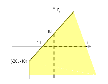
General Sensitivity Region for RHS's Values
Notice that, the sensitivity region contains the origin which corresponds to the nominal problem. Furthermore the vertex of the sensitivity region is at the point (-20, -10) where both RHS's vanish.
The shadow prices are the solution to the dual problem:
Min 20U1 + 10U2
subject to:
U1 + U2 ³ 2
3U1 + 5U2 ³ 4
2U1 ³ 3
U1 unrestricted, U2 £ 0.
As we already find, the optimal solution is: U1 = 2, and U2 = 0, with optimal value of 40 equal to the optimal value of the primal problem, as expected.
The binding constraints are:
U1 + U2 ³ 2
U2 £ 0.
Their RHS parametric version is:
U1 + U2 ³ 2 + c1
U2 £ 0.
The parametric optimal solution is:
U1 = 2 + c1
U2 = 0.
The parametric objective function is:
20U1 + 10U2 = 40 + 20c1 + 0c2 + 0c3
The solution to the dual of the dual (i.e., the primal) is X1 = 20, X2 = 0, and X3 =0, with optimal value of 40, as expected.
The dual parametric optimal solution is valid provided the parametric optimal solution satisfies the unused RHS parametric constraints, namely:
3U1 + 5U2 ³ 4 + c2
2U1 ³ 3 + c3
This reduces to:
3c1 - c2 ³ -2
2c1 - c3 ³ -1
This is the largest sensitivity region for the cost coefficients. This region, unlike the ordinary sensitivity analysis, allows us any simultaneous dependent or independent changes on the cost coefficients.
The individual cost coefficients sensitivity range is:
Construction of Simplex Final Tableau: To start the process of generating the simplex final tableau, the LP problem must be converted into the following standard form:
- Must be a maximization problem,
- RHS must be non-negative,
- All variables must be non-negative.
Notice that for equality constraint we introduce a dummy slack to obtain its RHS shadow price, Alternatively, we could convert all inequality constraints (except the non-negativity conditions) into equalities by introducing slack/surplus variables:
X1 + 3X2 + 2X3 + S1 = 20,
X1 + 5X3 - S2 = 10,
All variables are non-negative.
Since this problem has a non-degenerate unique optimal solution, i.e., X1 = 20, X2 = 0, X3 = 0, S1 = 0, S2 = 10, it is possible to generate the final simplex tableau. Notice that there are as many non-zero variables as the number of constraints which are two. Therefore, the basic variables are X1 = 20, and S2 = 10. The following is a “working tableau” for this problem:
| BVS | X1 | X2 | X3 | S1 | S2 | RHS | |
|---|---|---|---|---|---|---|---|
| X1 | 1 | 3 | 2 | 1 | 0 | 20 | |
| S2 | 1 | 5 | 0 | 0 | -1 | 10 | |
| Cj | 2 | 4 | 3 | 0 | 0 | 0 |
Using Gauss-Jordan row operation, the columns of X1 and S2 should be converted into:
| BVS | X1 | X2 | X3 | S1 | S2 | RHS | |
|---|---|---|---|---|---|---|---|
| X1 | 1 | 0 | 20 | ||||
| S2 | 0 | 1 | 10 | ||||
| Cj | 0 | 0 | -40 |
To obtain the final simplex tableau one need to perform Gauss-Jordan row operation including the last row by pivoting on column of X1 then column of S2, using the working tableau. Notice that since we include the row Cj in the row operation process, there is no need of, the row Zj, and the Cj-Zj, as are required by the simplex method. This greatly simplifies the construction of the final simplex tableau.
Pivoting on column of X1 we obtain:
| BVS | X1 | X2 | X3 | S1 | S2 | RHS | |
|---|---|---|---|---|---|---|---|
| X1 | 1 | 3 | 2 | 1 | 0 | 20 | |
| S2 | 0 | 2 | -2 | -1 | -1 | -10 | |
| Cj | 0 | -2 | -1 | -2 | 0 | -40 |
Finally pivoting on the column of S2, which in our case is obtained by simply multiplying the row S2 by -1:
| BVS | X1 | X2 | X3 | S1 | S2 | RHS | |
|---|---|---|---|---|---|---|---|
| X1 | 1 | 3 | 2 | 1 | 0 | 20 | |
| S2 | 0 | -2 | 2 | 1 | 1 | 10 | |
| Cj | 0 | -2 | -1 | -2 | 0 | -40 |
For larger problems one may use the JavaScript Solving Linear Parametric RHS System of Equations. In order to obtain the last row of the final simplex tableau, i.e., row Cj, one must introduce an identity column vector Cj row, as shown in the following table:
| BVS | X1 | X2 | X3 | S1 | S2 | Cj | RHS | |
|---|---|---|---|---|---|---|---|---|
| X1 | 1 | 3 | 2 | 1 | 0 | 0 | 20 | |
| S2 | 1 | 5 | 0 | 0 | -1 | 0 | 10 | |
| Cj | 2 | 4 | 3 | 0 | 0 | 1 | 0 |
Enter the columns of X1, S2 and Cj as the first three columns of the JavaScript data, followed by the rest of columns. You will obtain the following table, excluding the column of Cj from the output of the JavaScript, we obtain the following final simplex tableau:
| BVS | X1 | X2 | X3 | S1 | S2 | RHS | |
|---|---|---|---|---|---|---|---|
| X1 | 1 | 3 | 2 | 1 | 0 | 20 | |
| S2 | 0 | -2 | 2 | 1 | 1 | 10 | |
| Cj | 0 | -2 | -1 | -2 | 0 | -40 |
Note that by multiplying the last row of the final tableau by -1, it provides the shadow prices under columns of slack/surplus and the upper cost coefficient sensitivity limits for non-basic decision variables, i.e. for X2 and X3 are 2 and 1, respectively. , together with the optimal value which is 40.
Concluding Remarks: If a Linear Program (LP) has a finite optimal solution, it is one of Basic Feasible Solution (BFS). The importance of this fundamental theorem is that it reduces the LP problem to a "combinatorial" problem that of determining which constraints out of many should be satisfied by the optimal solution. The usual algebraic simplex method keeps trying different combinations and computing the objective function for each trial, until we find the best.
We presented a simple but general framework to solve LP problems manually, in an effective and efficient manner without using any slack/surplus variables or introducing new variables to restrict the sign of the unrestricted variables. All the variables are natural parts of the LP problem which are the decision variables (Xj). Our goal is a geometrically intuitive and broad simplification of finding BVS as well as an advance in classroom teaching.
The new algorithm is most suitable for LP problems with a large number of unrestricted variables, such as the dual problem of classical network models, Arsham [1995], and for problems where n and m are almost of the same magnitude.
In a short summary, we provide a simple algorithm which is an improved algebraic method contains the following nice features:
- It is an algebraic approach to solve a system of inequalities that provides a bridge between the graphical method and the simplex method, the LP software.
- It works within the decision variable space; no additional variables such as slack/surplus/artificial variables are added.
- It provides all information that the simplex method provides; such as shadow prices.
- It competes with LP software providing slack/surplus and sensitivity region and ranges for the RHS of the constraints and the coefficients of the objective function.
- It provides tight bounds on the objective function subject.
- It is free from degeneracy which may cause cycling.
- It is easy to understand, easy to apply and provides useful information to the decision maker. It is also valuable as a teaching tool.
Notice that the construction of the sensitivity regions presented here work well for LP with non-degenerate unique optimal solution. For these special cases, visit the following Web site: Construction of the Sensitivity Region for LP Models
Some areas for future research include looking for possible refinements, developments of an efficient code for performing a comparative computational study with other LP solvers. A convincing evaluation would be the application of this approach to a problem that has been solved by any other method.
Further Readings:
Adams W., Gewirtz A., and L. Quintas, Elements of Linear Programming, Van Nostrand Reinhold Co., New York, N.Y., 1969.
Arsham H., Links Among a Linear System of Equations, Matrix Inversion, and Linear Program Solver Routines, Journal of Mathematical Education in Science and Technology, 29(5), 764-769, 1998.
Arsham H., Postoptimality analyses of the transportation problem, Journal of The Operational Research Society, 43(1), 121-139, 1992.
Arsham H., A comprehensive simplex-like algorithm for network optimization and perturbation analysis, Optimization, 32(1), 211-267, 1995.
Arsham H., et. al., A Simplified Algebraic Method for System of Linear Inequalities with LP Applications, Omega: International Journal of Management Science, 37(4), 876-882, 2009.
Bradley S., A. Hax and T. Magnanti, Applied Mathematical Programming, Addison-Wesley, Reading, Mass., 1977.
Dantzig G., Linear Programming and Extensions, Princeton University Press, NJ., 1968.
Dantzig G. . Making progress during a stall in the simplex algorithm, Linear Algebra and Its Applications, 114(1) , 251-259, 1989.
Foldes S., Fundamental Structures of Algebra and Discrete Mathematics, Wiley, New York, NY., 1994.
Klee V. and Minty G., How good is the simplex algorithm, in Inequalities-III, Ed. Shisha O., Academic Press, New York, N.Y., 159-175, 1972.
Taha H., Integer Programming, Academic Press, New York, NY., 1975.
Winston W., Introduction to Mathematical Programming, Duxbury Press, 1995.
A Gradient Pivotal Solution Algorithm
1. Introduction:The simplex method is a well-known and widely used method for solving LP problems. The number of iterations needed to solve an LP by the simplex method depends mainly upon the pivot columns used, and can be exponential for certain LP problems.
The following section presents an efficient gradient-based algorithm for solving the general linear programming (LP) problem. The algorithm consists of three phases. The initialization phase provides the initial tableau which may not have a full set of basis. The push phase uses a full gradient vector of the objective function to obtain a feasible vertex. This is then followed by a series of pivotal steps using the sub-gradient, which leads to an optimal solution (if one exists) in the final iteration phase. At each of these iterations, the sub-gradient provides the desired direction of motion within the feasible region. The algorithm works in the space of the original variables. The algorithm hits and/or moves on the constraint hyper-planes and their intersections to reach an optimal vertex (if one exists). The computations are based on Gauss-Jordan pivoting as used in the simplex method, but the decision variables are allowed to be unrestricted. Therefore, there is no need to introduce new extra variables, and it is free of artificial variables.
2. The Solution Algorithm: General LP Problems:
Consider the following general linear programming problem:
Problem GLP:
Maximize C T
X
Subject To:
A 1
X £ b 1
A 2
X ³ b 2
where CÎ R n , [A1 , A 2 ] T ÎRmxn, (b 1 , b 2 ) T Î R m , and b 1 > 0, b 2 ³ 0.
We assume that [A 1 , A 2 ] T has a full row rank. Any restricted variable constraints are included in this set of constraints. Note that if there is an unrestricted variable in an equality constraint, one may use the constraint equation to eliminate the variable everywhere. This reduces the size of problem in both number of variables and number of constraints. Otherwise, convert each equality constraint into two inequality constraints. We assume that there are m constraints after all such transformations.
2.1. Intuitive description of the algorithm:
The basic idea is to start at the origin and utilize the full gradient of the objective function to get the first hit into the feasible region. We explain the process using the following problem:
Maximize z = 3X 1 + 5X2
Subject to:
2X1 + X £ 40,
X1 + 2X2 £ 50,
X 1 ³ 0, X 2 ³ 0.
In practical terms, we may suppose that the given problem represents profit maximization, subject to two capacity restrictions (e.g. machine-hours on different machines). The feasible region and gradient vector are shown in Figure 1. If the inequality sign of a constraint is replaced by an equality sign, a straight line (hyper-plane) is obtained which forms the boundary of the half space. If the problem is to be solved geometrically, the straight line z = 3X 1 + 5X 2 for an arbitrary value z is perpendicular to the gradient vector. The optimal z belongs to an iso-objective function line value which passes through a feasible vertex with the largest distance from the origin, which is 130. The hit points of the gradient vector with the constraints hyper-plane.
If we move in the direction of the full gradient in search of optimal vertex, this search strikes a boundary hyper-plane to get the first hit, which may or may not feasible. If a constraint hyper-plane is hit, the algorithm would not hit it again. Its path is then restricted to the boundary hyper-planes and their intersection and it continues on in such a manner that at each point it is moving in the direction of the updated full gradient of the objective function; namely that direction which takes it to feasibility and then to the optimal increase of the objective value. Once feasible, we reduce the dimensionality of the gradient space at each step and get closer to the optimal solution. The unique path defined by the starting point consists of a finite number of directional line segments (i.e., vectors) that provides the coordinates of the optimal vertex.
2.2. Development of gradient-based algorithm
Following are some additional notations used in the new gradient pivotal-based algorithm, hereafter referred to as Algorithm GP:
BVS = basic variable set
PR = pivot row
PC = pivot column
PE = pivot element
S i = the ith slack/surplus variable, 1£ i £ m
R i = the ith row of a tableau, 1£ i £ m
OR = open row, not yet assigned in the BVS
? = label for an open row
Ck = vector of the last row of the kth tableau
Zk = vector { Zkj : Zkj = Ckj for 1 £ j £ n, Zkj = 0 for j > n}
C k + = vector { Ckj + : Ckj + = Ckj if Ckj ³ 0, Ckj + = 0 otherwise}
N(Ck +
) = the number of positive entries in vector Ck +
RHS = right hand side
Yk = the kth inner product of two vectors
L = column ratios, RHS/Yk
The algorithm consists of an initialization phase, a push phase, and a final iteration phase of sequential pivoting, to reach an optimal solution.
Algorithm GP
Initialization Phase
Step I1: Convert the LP to the standard form GLP.
Step I2: Introduce slack/surplus variables for each constraint.
Step I3: Initialize k = 1.
rgradra54 Set up the initial simplex tableau by keeping rows for all £ constraints, except for the non-negativity constraints, open.
To start the algorithm the LP should be converted to the standard form of problem GLP with all £ inequalities with positive RHS. Any constraint with 0 in the RHS, except for non-negativity constraints, should appear as a ³ inequality only. The non-negativity constraints should be converted to £ inequalities to add the slack variables. The rows for these constraints are not open. This phase sets the origin as the starting point. Note that by this construction all slack variables would appear in the initial BVS. If all constraints are £ inequalities, there will be no open row. This implies that the push phase is not needed.
Push Phase
Step P1: Check if a (?) label exists in the BVS. If no, go to step F1.
Step P2: Create column Yk as inner product of each row with Zk, Yki= Zk × Ri .
Step P3: Save non-zero Zkj's as C k (X j ) = Zkj.
Step P4: Create vector L of column ratios.
Step P5: If Li < 0 for all OR’s, go to Step P7.
Step P6: Determine step length as L l = min { Li : Ri is OR, Ll ³ 0}. Set PE = Ykl . Go to Step P8.
Step P7: Determine step length as L l = min { |Li |: Ri is OR}. Set PE = Y kl .
Step P8: Perform GJP on the kth tableau. Adjust the BVS.
Step P9: Set k ® k+1. Go to step P1.
The purpose of this phase is to complete the BVS of the initialization phase while moving in the direction of the full gradient to get some hits on a boundary hyper-plane. The variables are brought into open rows marked by (?) only, and there is no replacement of variables in the BVS. Thus, in this phase, we push toward a basic feasible solution.
Let the starting point, the origin, be denoted by X0 , which may be an incomplete basic solution already available in tabular form. Starting at X0 , the algorithm moves in the direction of the full-gradient whose elements are the elements of C1 . Find the first hyper-plane which is a hit with the smallest non-negative step size. If all eligible entries are negative, we take the smallest absolute step size. Let the hit point be X1 . Pivot on X1. Continue till the BVS is complete, indicating a hit Xk with a feasible hyper-plane. If by the end of this phase, Ck £ 0, this is an optimum solution.
Final Iteration Phase
Step F1: If C kj £ 0 for all j, go to Step F10.
Step F2: Create column Y k as inner product of each row with C k + , Y ki = C k + × R i
Step F3: Save C ki + 's as C k (X j ) = C kj + .
Step F4: Create vector L of column ratios.
Step F5: Determine the permissible step length as L l = min { L i : L i ³ 0, 1£ i £ m}. Set PR = l.
rgradra54 Set PE = Y kl .
Step F7: Perform GJP on the k th tableau. Set k ® k+1. Adjust the BVS.
Step F8: If N(C k +
) < N(C k-1 +
), go to Step F1.
Step F9: Set k ® k-1, delete the lth
row from the kth
tableau. Go to Step F1.
Step F10: STOP. The tableau is optimal. Construct optimal solution.
The purpose of this phase is to reach to an optimal vertex while maintaining feasibility. Starting from X k move toward the sub-gradient whose elements are C k + . This pivot gives a hit point X k+1 . One of two distinct cases arises:
- The order of gradient reduces (i.e. the number of positive entries in C k + never increase): implies that the hit hyper-plane contains an optimal solution. Use X k+1 as the new starting point. Continue with the new sub-gradient to search for a new hit. The working space of the problem is now in this reduced space. The intersection of this hyper-plane with its adjacent hyper-planes provides the boundaries of the new feasible region.
- The order of gradient remains the same (i.e. the number of positive C k + remains the same): implies that the hit hyper-plane does not contain an optimal solution. Starting from X k+1 move along the new sub-gradient to find a new hit. Delete the hyper-plane of the previous hit. This reduces the size of the problem and prevents the zigzagging.
The optimal solution, X j * for 1 £ j £ n, are obtained using the final tableau as follows:
Where S is over all values of k, and l(Yk) = 1 if Yk is in BVS, l(Yk) = 0 otherwise. The needed information to compute Xj* is extracted at the end of each tableau to avoid saving the whole tableau. This saves storage as, like the simplex method, we only need the current tableau to generate the next one. Compute slack/surplus values in the same manner, or use the original constraints, using the optimal solution of the decision variables set X* .
2.3. Notes for Algorithm GP
- If all constraints of an LP are £ inequalities with RHS > 0 and C > 0, a feasible hit is certain and the push phase is bypassed. Non-negative constraints may be present.
- The first tableau provides a BVS which may not be complete, but always provides the origin as an initial starting point.
- In the push phase, to ensure the first hit we use the full gradient direction which has n components. The strategy is to get on a feasible boundary hyper-plane via gradient direction. In the process, we may get a hit outside of the feasible boundary hyper-plane, i.e., RHS may become negative. At the end of this phase, a basic feasible solution is available. The push phase can be viewed as a gradient pivotal phase.
- The Yk column is always the PC. The smallest step size determines the PR, hence PE is always in the Yk column, and only Yk ’s can come into the BVS.
- In the final iteration phase we restrict ourselves to only positive entries of Ck , the last row of kth tableau, and use the vector Ck + to determine the sub-gradient direction (which is a feasible direction) at each step of iteration to ensure improvement.
- The final iteration phase maintains feasibility hence all slack/surplus variables should maintain non-negative RHS. Negative slack/surplus is a sign of infeasibility. Yk ’s can have negative RHS.
- The number of positive entries in Ck either remains the same or reduces. This is unlike the simplex method where this number may increase from any iteration to the next.
- At each iteration, before a new tableau replaces the old one, we save the Ck entries used in the inner product to create Yk . These entries are used later to construct optimal values of the variables. This saves the storage requirement as in the simplex method.
- The algorithm terminates when all elements of a Ck row are non-positive and all RHS for slacks are ³ 0. As will be discussed latter, the algorithm also discovers if the problem is unbounded or infeasible.
- The simplex method brings one column at a time into the BVS. The Algorithm GP brings Y k , which is constructed using many eligible columns, into the basis at each step. Thus it combines several variables at each step.
- If any unrestricted variable, X j , appears in an equality constraint, one may use the constraint equation to eliminate X j from the problem and reduce the size of the problem in both number of variables and number of constraints. Otherwise, convert each equality constraint to two inequality constraints to force the gradient direction to hit either of corresponding hyper-plane so that these constraints are satisfied at every subsequent steps.
- Combining both the deletion and the inclusion of the original hyper-planes of the boundary of the feasible region, together with the fact that the gradient vector, if it hits a hyper-plane, hits it once only, we never return to the same hyper-plane. For this reason there is no zigzagging precaution and, thus, finiteness follows. The amount of computation per iteration required by the proposed algorithm is insignificantly greater than that required by the standard simplex method. The algorithm is also robust with respect to gradient data perturbation.
- The algorithm is most suitable for problems with m >> n. Otherwise one may solve the dual by the proposed algorithm, and then use the complementary slackness theorem to compute the optimal solution of the original (primal) problem.
3. Illustrative Examples and Computational Aspects:
The following examples are to demonstrate various steps and computational aspects of Algorithm GP
Problem P1:
Maximize 2X2 + 3X2
Subject to:
X1 + 2X2 £ 8,
2X1 + X2 £ 10,
X2 £ 7/2,
X1 £ 4
Since all constraints are £ inequalities, Algorithm GP would take at most m = 4 iterations to solve this LP.
Initialization Phase: After performing steps 1 thru 4, we obtain the initial tableau.
| BVS | X1 | X2 | S1 | S2 | S3 | S4 | Y1 | RHS | L | |
|---|---|---|---|---|---|---|---|---|---|---|
| S1 | 1 | 2 | 1 | 0 | 0 | 0 | 8 | 8 | 1 | |
| S2 | 2 | 1 | 0 | 1 | 0 | 0 | 7 | 10 | 10/7 | |
| S3 | 0 | 1 | 0 | 0 | 1 | 0 | 3 | 7/2 | 7/6 | |
| S4 | 1 | 0 | 0 | 0 | 0 | 1 | 2 | 4 | 2 | |
| C1 | 2 | 3 | 0 | 0 | 0 | 0 | 13 |
Note that there is no open (?) row, since there is no constraint with ? inequality. Hence the push phase is not needed. Final Iteration Phase: Calculate Y1 and L (column/row ratios). Y1 uses C1 (X1) = 2, and C1 (X1) = 3. Save this information. To avoid redundancy of calculations, we add Y1 and L columns to the previous tableau. From now on this will be the standard way of placing these columns. Since L1 = 1 is the smallest ratio, and the C1 row has the largest positive number in the Y1 column, PE = Y11 , perform GJP.
| BVS | X1 | X2 | S1 | S2 | S3 | S4 | Y1 | Y2 | RHS | L | |
|---|---|---|---|---|---|---|---|---|---|---|---|
| Y1 | 1/8 | 2/8 | 1/8 | 0 | 0 | 0 | 1 | 3/64 | 1 | 64/3 | |
| S2 | 9/8 | -6/8 | -7/8 | 1 | 0 | 0 | 0 | 27/64 | 3 | 64/9 | |
| S3 | -3/8 | 2/8 | -3/8 | 0 | 1 | 0 | 0 | -9/64 | 1/2 | -- | |
| S4 | 6/8 | -4/8 | -2/8 | 0 | 0 | 1 | 0 | 18/64 | 2 | 64/9 | |
| C2 | 3/8 | -10/8 | -13/8 | 0 | 0 | 0 | 0 | 9/64 |
We continue to calculate Y2 and L columns in the same tableau after performing GJP. Save C2 (X1) = 3/8. Looking at the positive L entries for a possible step length, we find a tie. We randomly pick S4 to exit. Perform the GJP (see the tables).
| BVS | X1 | X2 | S1 | S2 | S3 | S4 | Y1 | Y2 | RHS | |
|---|---|---|---|---|---|---|---|---|---|---|
| Y1 | 0 | 1/3 | 1/6 | 0 | 0 | -1/6 | 1 | 0 | 2/3 | |
| S2 | 0 | 0 | -1/2 | 1 | 0 | -3/2 | 0 | 0 | 0 | |
| S3 | 0 | 1 | -1/2 | 0 | 1 | 1/2 | 0 | 0 | 3/2 | |
| Y2 | 8/3 | -16/9 | -8/9 | 0 | 0 | 32/9 | 0 | 1 | 64/9 | |
| C3 | 0 | -1 | -3/2 | 0 | 0 | -1/2 | 0 | 0 |
The result is optimal tableau, as there is no positive entry in the C3 row. Note that this tableau is not like the usual simplex tableau and there is no basis inverse nor a dual solution. By knowing the optimal solution, clearly, these can be computed by inverting the optimal basis matrix and using the complementary slackness theorem respectively. The optimal solution can be found by using the information saved at the end of each iteration on Yj and the final tableau, as follows:
X1 = 0 + 2(2/3) + 3/8 (64/9) = 4
X2 = 0 + 3(2/3) = 2
S1 = 0, S2 = 0, S3 = 3/2, S4 = 0.
Problem P2:
Maximize 2X1 + 2X2
Subject To:
X1 + X2 ³ 1,
X1 + X2 £ 2,
-2X1 + X2 ³ 0,
X1 ³ 0, X2
unrestricted
There are 2 ³ inequalities and 4 constraints. Thus, Algorithm GP would need 2 iterations in the push phase and at most 4 iterations in the final iteration phase.
Initialization Phase: Add slack and surplus variables. Note that we do not introduce any artificial variables. Construct the initial tableau by keeping the rows for the first and third constraints open.
| BVS | X1 | X2 | S1 | S2 | S3 | S4 | Y1 | RHS | L | |
|---|---|---|---|---|---|---|---|---|---|---|
| ? | -1 | -1 | 1 | 0 | 0 | 0 | -4 | -1 | 1/4 | |
| S2 | 1 | 1 | 0 | 1 | 0 | 0 | 4 | 2 | -- | |
| ? | -2 | 1 | 0 | 0 | -1 | 0 | -2 | 0 | 0 | |
| S4 | -1 | 0 | 0 | 0 | 0 | 1 | -2 | 0 | -- | |
| C1 | 2 | 2 | 0 | 0 | 0 | 0 | 8 |
Push Phase: After obtaining the tableau, we introduce Y1 . Save C1 (X1) = 2 and C1 (X2) = 2. In this phase we can allow RHS to become negative because it is possible to hit outside the feasible region in the process of reaching it. We consider column L entries for open rows only. After GJP on Y13, we get the next tableau presented below.
| BVS | X1 | X2 | S1 | S2 | S3 | S4 | Y1 | Y2 | RHS | L | |
|---|---|---|---|---|---|---|---|---|---|---|---|
| ? | -3 | 3 | -1 | 0 | -2 | 0 | 0 | 36 | 1 | 1/36 | |
| S2 | -3 | 3 | 0 | 1 | -2 | 0 | 0 | 36 | 2 | -- | |
| Y1 | 1 | -1/2 | 0 | 0 | 1/2 | 0 | 1 | -9 | 0 | -- | |
| S4 | 1 | -1 | 0 | 0 | 1 | 1 | 0 | -12 | 0 | -- | |
| C2 | -6 | 6 | 0 | 0 | -4 | 0 | 0 | 72 |
Create Y2 . Save C2 (X1) = -6 and C2 (X2) = 6. The next iteration completes the BVS.
| BVS | X1 | X2 | S1 | S2 | S3 | S4 | Y1 | Y2 | Y3 | RHS | L | |
|---|---|---|---|---|---|---|---|---|---|---|---|---|
| Y2 | -1/12 | 1/12 | -1/36 | 0 | -1/18 | 0 | 0 | 1 | -1/18 | 1/36 | -1/2 | |
| S2 | 0 | 0 | 1 | 1 | 0 | 0 | 0 | 0 | 2 | 1 | 1/2 | |
| Y1 | 1/4 | 1/4 | -1/4 | 0 | 0 | 0 | 1 | 0 | -1/2 | 1/4 | -1/2 | |
| S4 | 0 | 0 | -1/3 | 0 | 1/3 | 1 | 0 | 0 | -2/3 | 1/3 | -1/2 | |
| C3 | 0 | 0 | 2 | 0 | 0 | 0 | 0 | 0 | 4 |
Final Iteration Phase: Again, we add columns Y3 and L in the previous tableau. Perform GJP.
| BVS | X1 | X2 | S1 | S2 | S3 | S4 | Y1 | Y2 | Y3 | RHS | |
|---|---|---|---|---|---|---|---|---|---|---|---|
| Y2 | -1/12 | 1/12 | 0 | 1/36 | -1/18 | 0 | 0 | 1 | 0 | 1/18 | |
| Y3 | 0 | 0 | 1/2 | 1/2 | 0 | 0 | 0 | 0 | 1 | 1/2 | |
| Y1 | 1/4 | 1/4 | 0 | 1/4 | 0 | 0 | 1 | 0 | 0 | 1/2 | |
| S4 | 0 | 0 | 0 | 1/3 | 1/3 | 1 | 0 | 0 | 0 | 2/3 | |
| C4 | 0 | 0 | 0 | -2 | 0 | 0 | 0 | 0 | 0 |
This is the optimal solution. The solution is:
Note: There is no reduction in the dimension of the gradient when we move from tableau 2 (with C2) to tableau 3 (with C3). This indicates that the first constraint is never a binding constraint. So, as per step F9, we could go back to the previous tableau deleting the first constraint. Recall that this step reduces the complexity of the LP and eliminates zigzagging among hits. The adjusted tableau is shown below.
| BVS | X1 | X2 | S2 | S3 | S4 | Y1 | Y2 | RHS | L | |
|---|---|---|---|---|---|---|---|---|---|---|
| S2 | -3 | 3 | 1 | -2 | 0 | 0 | 18 | 2 | 1/9 | |
| Y1 | 1 | -1/2 | 0 | 1/2 | 0 | 1 | -3 | 0 | - | |
| S4 | 1 | -1 | 0 | 1 | 1 | 0 | -6 | 0 | - | |
| C2 | -6 | 6 | 0 | -4 | 0 | 0 | 36 |
Final Iteration Phase: Note that in this phase, like in simplex, only those 0 values are permissible in L where RHS = 0 and the corresponding PC value is positive. Calculate Y2 and L. Save C2 (X2 ) = 6. Performing GJP on Y21 yields:
| BVS | X1 | X2 | S2 | S3 | S4 | Y1 | Y2 | RHS | |
|---|---|---|---|---|---|---|---|---|---|
| Y2 | -1/6 | 1/6 | 1/18 | -1/9 | 0 | 0 | 1 | 1/9 | |
| Y1 | 1/2 | 0 | 1/6 | 1/6 | 0 | 1 | 0 | 1/3 | |
| S4 | 0 | 0 | 1/3 | -1/3 | 1 | 0 | 0 | 2/3 | |
| C3 | 0 | 0 | -2 | 0 | 0 | 0 | 0 |
This is the optimal tableau with solution:
Problem P3:
Maximize -X1 - X2
Subject To:
2X1 + X2 ³ 4,
X1 + 2X2 ³ 5
Algorithm GP takes at most 2m = 4 iterations (if successful) to solve problem P3.
| BVS | X1 | X2 | S1 | S2 | Y1 | RHS | L | |
|---|---|---|---|---|---|---|---|---|
| ? | 2 | 1 | -1 | 0 | -3 | 4 | -4/3 | |
| ? | 1 | 2 | 0 | -1 | -3 | 5 | -5/3 | |
| C1 | -1 | -1 | 0 | 0 | 2 |
Push Phase: Now, PC = Y1. Save C1 (X1) = -1 and C1 (X2) = -1. Since Li < 0 for all i, this indicates that the full gradient direction is away from the feasible region. By determining PE as in Step P6, we change the direction to get a first hit. Also notice that C1 < 0 is not an indication of optimality. In this sense, the initial tableau and the subsequent iterative tableaux differ in characteristics. The table is obtained:
| BVS | X1 | X2 | S1 | S2 | Y1 | Y2 | RHS | L | |
|---|---|---|---|---|---|---|---|---|---|
| Y1 | -2/3 | -1/3 | 1/3 | 0 | 1 | -1/9 | -4/3 | -- | |
| ? | -1 | 1 | 1 | -1 | 0 | -2/3 | 1 | -3/2 | |
| C2 | 1/3 | -1/3 | -2/3 | 0 | 0 | 2/9 |
Create Y2. Save C2(X1) = 1/3 and C2(X2) = -1/3. Perform GJP on Y22
| BVS | X1 | X2 | S1 | S2 | Y1 | Y2 | RHS | |
|---|---|---|---|---|---|---|---|---|
| Y1 | -1/2 | -1/2 | 1/6 | 1/6 | 1 | 0 | -3/2 | |
| Y2 | 3/2 | -3/2 | -3/2 | 3/2 | 0 | 1 | -3/2 | |
| C2 | 0 | 0 | -1/3 | -1/3 | 0 | 0 |
This is the optimal tableau, so no iteration is needed in the final phase. The optimal solution is:
We consider the following problem as the worst possible case of a gradient direction.
Problem P4:
Maximize X1 - X2
Subject To:
X1 £ 10,
X1 £ 5,
X2 £ 10,
and X2 £ 5.
Maximum possible number of iterations = 6 (if successful). The following tableaux are obtained in succession:
| BVS | X1 | X2 | S1 | S2 | S3 | S4 | Y1 | RHS | L | |
|---|---|---|---|---|---|---|---|---|---|---|
| S1 | 1 | 0 | 1 | 0 | 0 | 0 | 1 | 10 | -- | |
| ? | 1 | 0 | 0 | -1 | 0 | 0 | 1 | 5 | 5 | |
| S3 | 0 | 1 | 0 | 0 | 1 | 0 | -1 | 10 | -- | |
| ? | 0 | 1 | 0 | 0 | 0 | -1 | -1 | 5 | -5 | |
| C1 | 1 | -1 | 0 | 0 | 0 | 0 | 2 |
| BVS | X1 | X2 | S1 | S2 | S3 | S4 | Y1 | Y2 | RHS | L | |
|---|---|---|---|---|---|---|---|---|---|---|---|
| S1 | 0 | 0 | 1 | 1 | 0 | 0 | 0 | 0 | 5 | -- | |
| Y1 | 1 | 0 | 0 | -1 | 0 | 0 | 1 | -1 | 5 | -- | |
| S3 | 1 | 1 | 0 | -1 | 1 | 0 | 0 | -2 | 15 | -- | |
| ? | 1 | 1 | 0 | -1 | 0 | -1 | 0 | -2 | 10 | -5 | |
| C2 | -1 | -1 | 0 | 2 | 0 | 0 | 0 | 2 |
| BVS | X1 | X2 | S1 | S2 | S3 | S4 | Y1 | Y2 | Y3 | RHS | L | |
|---|---|---|---|---|---|---|---|---|---|---|---|---|
| S1 | 0 | 0 | 1 | 1 | 0 | 0 | 0 | 0 | 1 | 5 | 5 | |
| Y1 | 1/2 | -1/2 | 0 | -1/2 | 0 | 1/2 | 1 | 0 | -1/2 | 0 | -- | |
| S3 | 0 | 0 | 0 | 0 | 1 | 1 | 0 | 0 | 0 | 5 | -- | |
| Y2 | -1/2 | -1/2 | 0 | 1/2 | 0 | 1/2 | 0 | 1 | 1/2 | -5 | -10 | |
| C3 | 0 | 0 | 0 | 1 | 0 | -1 | 0 | 0 | 1 |
Create Y3. Perform GJP on Y31
| BVS | X1 | X2 | S1 | S2 | S3 | S4 | Y1 | Y2 | Y3 | RHS | |
|---|---|---|---|---|---|---|---|---|---|---|---|
| Y3 | 0 | 0 | 1 | 1 | 0 | 0 | 0 | 0 | 1 | 5 | |
| Y1 | 1/2 | -1/2 | 1/2 | 0 | 0 | 1/2 | 1 | 0 | 0 | 5/2 | |
| S3 | 0 | 0 | 0 | 0 | 1 | 1 | 0 | 0 | 0 | 5 | |
| Y2 | -1/2 | -1/2 | -1/2 | 0 | 0 | 1/2 | 0 | 1 | 0 | -15/2 | |
| C4 | 0 | 0 | -1 | 0 | 0 | -1 | 0 | 0 | 0 |
This is the optimal tableau. The final solution is:
X1 = 0 + 1(5/2) + (-1)(-15/2) = 10, X2 = 0 + (-1)(5/2) + (-1)(-15/2) = 5, S1 = 0, S2 = 0, S3 = 5, S4 = 0.
4. Special Cases:
4.1. Unbounded solutions
Sometimes the feasible region of an LP is unbounded and the objective function can be made infinitely large without violating any of the constraints. In a manner similar to the simplex, this unboundedness of a problem is captured by Algorithm GP through the detection of the existence of a PC, i.e., Y4 , with all negative entries.
Problem P5:
Maximize X1 + X2
Subject To:
-X1 + X2 £ 1,
-2X1 + X2 £ 0
Starting from initialization, the following tableaux are obtained successively.
| BVS | X1 | X2 | S1 | S2 | Y1 | RHS | L | |
|---|---|---|---|---|---|---|---|---|
| S1 | -1 | 1 | 1 | 0 | 0 | 1 | -- | |
| ? | 2 | -1 | 0 | -1 | 1 | 0 | 0 | |
| C1 | 1 | 1 | 0 | 0 | 2 |
| BVS | X1 | X2 | S1 | S2 | Y1 | Y2 | RHS | L | |
|---|---|---|---|---|---|---|---|---|---|
| S1 | -1 | 1 | 1 | 0 | 0 | 3 | 1 | 1/3 | |
| Y1 | 2 | -1 | 0 | -1 | 1 | -5 | 0 | -- | |
| C2 | -1 | 3 | 0 | 2 | 0 | 13 |
| BVS | X1 | X2 | S1 | S2 | Y1 | Y2 | RHS | |
|---|---|---|---|---|---|---|---|---|
| Y2 | -1/3 | 1/3 | 1/3 | 0 | 0 | 1 | 1/3 | |
| Y1 | 1/3 | 2/3 | 5/3 | -1 | 1 | 0 | 5/3 | |
| C3 | 10/3 | -4/3 | -13/3 | 2 | 0 | 0 |
Note that there is no reduction in dimensionality (step F9). Drop the first constraint in the second tableau with C2. Again, Y2 is the entering variable, but has only a negative entry in its column, indicating unboundedness.
4.2. Infeasibility
Sometimes there is no solution that satisfies all the constraints of a problem. Algorithm GP identifies this as follows. Note that all entries under RHS corresponding to the slack variables must always be non-negative in all phases. The presence of a negative value at any time would indicate infeasibility.
Problem P6:
Maximize 2X1 + 2X2
Subject To:
X1 + X2 ³ 2,
X1 + X2 £ 1
The tables are shown below.
| BVS | X1 | X2 | S1 | S2 | Y1 | RHS | L | |
|---|---|---|---|---|---|---|---|---|
| ? | 1 | 1 | -1 | 0 | 4 | 2 | 1/2 | |
| S2 | 1 | 1 | 0 | 1 | 4 | 1 | -- | |
| C1 | 2 | 2 | 0 | 0 | 8 |
| BVS | X1 | X2 | S1 | S2 | Y1 | RHS | |
|---|---|---|---|---|---|---|---|
| Y1 | 1/4 | 1/4 | -1/4 | 0 | 1 | 1/2 | |
| S2 | 0 | 0 | 1 | 1 | 0 | -1 | |
| C1 | 0 | 0 | 2 | 0 | 0 |
This tableau has a slack variable, S2, with a negative RHS, indicating infeasibility.
4.3. Alternate/multiple solutions
An LP problem on occasion may have two or more alternate optimal solutions. The proposed algorithm provides a clear indication of the presence of alternative optimal solutions upon termination. The decision-maker now has the option of deciding which optimal solution to implement on the basis of other factors involved. Like the simplex method, an LP has multiple solutions if at least one of the Ck entries for the non-basic variables is zero.
Problem P7:
Maximize 2X1 + 2X2
Subject To:
-X1 + X2 £ 1,
X1 + X2 £ 2,
X1 - X2 £ 1
Here m=3, therefore we need at most 3 iterations (if successful). However, we get the optimal tableau after only one iteration.
| BVS | X1 | X2 | S1 | S2 | S3 | Y1 | RHS | L | |
|---|---|---|---|---|---|---|---|---|---|
| S1 | -1 | 1 | 1 | 0 | 0 | 0 | 1 | -- | |
| S2 | 1 | 1 | 0 | 1 | 0 | 4 | 2 | 1/2 | |
| S3 | 1 | -1 | 0 | 0 | 1 | 0 | 1 | -- | |
| C1 | 2 | 2 | 0 | 0 | 0 | 8 |
| BVS | X1 | X2 | S1 | S2 | S3 | Y1 | RHS | |
|---|---|---|---|---|---|---|---|---|
| S1 | -1 | 1 | 1 | 0 | 0 | 0 | 1 | |
| Y1 | 1/4 | 1/4 | 0 | -1/4 | 0 | 1 | 1/2 | |
| S3 | 1 | -1 | 0 | 0 | 1 | 0 | 1 | |
| C1 | 0 | 0 | 0 | -2 | 0 | 0 |
This is an optimal tableau. The zeros in the C2 row for non-basic variables X1 and X2 indicate a presence of multiple solutions. The optimal solution from this tableau is X1 = 1, X2 = 1. Since S1 = 1, and S3 = 1, we have more positive variables than the number of constraints, indicating that the optimal solution is not at a vertex. To generate the two vertices, bring in X1in the above tableau to get X1 = 3/2, X2 = 1/2; or, bring in X2 to get X1 = 1/2, X2 = 3/2.
4.4. Treatment of Degeneracy
Degeneracy is a phenomenon that can arise in the simplex method. If it does arise, it certainly influences any vertex-searching method. However, Algorithm GP is not a vertex-searching method. Therefore, degeneracy is a very rare occurrence in the searching of an optimal solution. If it occurs, one can perturb the component of the gradient by e procedure or take any other anti-degeneracy precaution which works for the simplex method.
Further Readings:
Arsham H., An interior pivotal solution algorithm for linear programs,
Applied Mathematics and Computation Vol. 188, No. 1, 596-611, 2007
Arsham H., A combined gradient and feasible direction pivotal solution algorithm for general LP,
Revista Investigacion Operational, Vol. 19, No. 1, 3-19, 1998.
Which Solution Algorithm Is the Best?
Further Readings:
Klee V., and G. Minty, How good is the simplex algorithm, in Inequalities-III, Edited by O. Shisha, Academic Press, 1972, 159-175.
Goal-Seeking Problems
In most real-life situations the decision maker may not be interested in optimization but wishes to achieve a certain value for the objective function. Most managers are satisfied with a "good enough" solution. This problem is referred to "satisfying" the "goal-seeking" problem.Some parts of the reason business manager overestimate the importance of optimal strategy is that organizations often use indicators as "proxies" for satisfying their immediate needs. Most managers pay attention to indicators, such as profit, cash flow, share price etc., to indicate survival than as a goal for optimization.
To solve the goal-seeking problem one must first add the goal as part of the constraint set. To convert the goal seeking problem to an optimization problem one must create a dummy objective function. It could be a linear combination of the sub-set of decision variables. If you maximize this objective function, you will get a feasible solution (if one exists). If you minimize it, you will maybe get another one (usually at the other "side" of the feasible region). You could optimize with different objective functions.
Another approach is to use "Goal Programming" models, which deal precisely with problems of constraint satisfaction without necessarily having a single objective. Basically, they look at measures of constraint violation, and try to minimize these. You can formulate and solve goal programming models in ordinary LP, using ordinary LP solution codes.
In the artificial-free solution algorithms, one may use a zero dummy objective function but not in some software packages such as Lindo. In using software packages one may maximize or minimize any variable as an objective function.
Numerical Example
Consider Example 1 in the Initialization of the Simplex Method section of a companion site to this site. Suppose instead of maximizing, we now wish to achieve a goal of 4. That is,
Goal: -X1 + 2X2 = 4
subject to:
X1 + X2 ³ 2,
-X1 + X2 ³ 1,
X2 £ 3,
and X1, X2 ³ 0.
Adding this goal to the constraint set, and converting the constraints into equality form, we have:
X1 + X2 - S1 = 2, -X1 + X2 - S2 = 1, X2 + S3 = 3, and
X1, X2, S1, S2, S3 ³ 0.
The initial tableau for this problem, with dummy objective function of 0, is:
| BVS | X1 | X2 | S1 | S2 | S3 | RHS | C/R | |
|---|---|---|---|---|---|---|---|---|
| ? | (1) | 1 | -1 | 0 | 0 | 2 | 2/1 | |
| ? | -1 | 1 | 0 | -1 | 0 | 1 | -1/1 | |
| ? | 0 | 1 | 0 | 0 | 1 | 3 | --- | |
| ? | -1 | 2 | 0 | 0 | 0 | 4 | -4/1 | |
| Cj | 0 | 0 | 0 | 0 | 0 | 0 |
X1 comes in. The next tableau is:
| BVS | X1 | X2 | S1 | S2 | S3 | RHS | C/R | |
|---|---|---|---|---|---|---|---|---|
| X1 | 1 | 1 | -1 | 0 | 0 | 2 | 2/1 | |
| ? | 0 | (2) | -1 | -1 | 0 | 3 | 3/2 | |
| ? | 0 | 1 | 0 | 0 | 1 | 3 | 3/1 | |
| ? | 0 | 3 | -1 | 0 | 0 | 6 | 6/3 | |
| Cj | 0 | 0 | 0 | 0 | 0 | 0 |
Similarly, bringing the other variables in the BV set, we get:
| BVS | X1 | X2 | S1 | S2 | S3 | RHS | C/R | |
|---|---|---|---|---|---|---|---|---|
| X1 | 1 | 0 | -1/2 | 1/2 | 0 | 1/2 | -1 | |
| X2 | 0 | 1 | -1/2 | -1/2 | 0 | 3/2 | -3 | |
| ? | 0 | 0 | (1/2) | 1/2 | 1 | 3/2 | 3 | |
| ? | 0 | 0 | 1/2 | -3/2 | 0 | 3/2 | 3 | |
| Cj | 0 | 0 | 0 | 0 | 0 | 0 |
The next tableau is:
| BVS | X1 | X2 | S1 | S2 | S3 | RHS | C/R | |
|---|---|---|---|---|---|---|---|---|
| X1 | 1 | 0 | 0 | 1 | 1 | 2 | 2 | |
| X2 | 0 | 1 | 0 | 0 | 1 | 3 | --- | |
| S1 | 0 | 0 | 1 | 1 | 2 | 3 | 3 | |
| ? | 0 | 0 | 0 | (-2) | -1 | 0 | 0 | |
| Cj | 0 | 0 | 0 | 0 | 0 | 0 |
And finally:
| BVS | X1 | X2 | S1 | S2 | S3 | RHS | |
|---|---|---|---|---|---|---|---|
| X1 | 1 | 0 | 0 | 0 | -1/2 | 2 | |
| X2 | 0 | 1 | 0 | 0 | 1 | 3 | |
| S1 | 0 | 0 | 1 | 0 | -3/2 | 3 | |
| S2 | 0 | 0 | 0 | 1 | 1/2 | 0 | |
| Cj | 0 | 0 | 0 | 0 | 0 | 0 |
A solution is X1 = 2, X2 = 3, S1 = 3, S2 = 0, and S3 = 0.
How to Solve ILP by LP Solvers? Cutting Plane Method
Suppose that we wish to solve the following Integer LP problem:
Max 14X1 + 30 X2
subject to:
7X1 + 16 X2 £ 52
3X1 -2X2 £ 9
and both decision variables must be non-negative integers.
The first step is to relax (i.e., ignore) the integrality condition and solve this problem as an LP. The result is X1 = 4, and X2 =3/2. This solution is not feasible for the ILP problem. The customary practical approach is to round the solution to the near integers, that is, X1 = 4, X2 = 1, or X1 = 4, X2 = 2. Unfortunately, none of these are even feasible for the ILP. Even, if any one of them were feasible, we are not sure that it is optimal. Therefore, an effective approach, which guarantee an optimal solution (if one exists) must be used. An effective approach is known as "The Cutting-Plane Method", which cuts off the feasible region to exclude the obtained non-integer variables one-by-one.
In the application of cutting plane method, initially, we ignore the integer condition by solving the problem as an LP problem, if the solution satisfies the integrality condition(s), we are done. Otherwise, we add a new constraint to exclude (to cut-off) this solution while including all the original feasible solutions. The following small numerical example illustrates the process.
Max 3X1 + 5X2
subject to:
X1 + 8/5X2 £ 4
both decision variables must be non-negative integers.
The first step is to make all coefficients in the problem integer, if necessary. Therefore, the equivalent ILP problem to this problem is:
Max 3X1 + 5X2
subject to:
5X1 + 8X2 £ 20
both decision variables must be non-negative integers.
Using the simplex method, we get the following final tableau:
| BVS | X1 | X2 | S1 | RHS | |
|---|---|---|---|---|---|
| X2 | 5/8 | 1 | 1/8 | 5/2 | |
| Cj | -1/8 | 0 | -5/8 |
Therefore, X1 = 0, X2 = 5/2. This solution is not integer, and if we round this solution, both results are feasible but not optimal, as we will find later. Therefore, we must introduce a cut.
In the final table, consider the row, which the RHS violates the integrality condition. Break any ties, arbitrarily. In this numerical example, we have to consider the first row (i.e., the only row) in the above table. Find out "the rounding-it down fraction" for each entries in that row. That is, the absolute-value of the fractional-number needed to round-down each entry in that row. Construct the cut. The cut is always a constraint of ³ form with all non-negative coefficients, including the RHS. For this problem, the cut is 5/8X1 + 1/8S1 ³ 1/2. Following the steps described in the Initialization of the Simplex Method with this added new constraint, we get the final tableau:
| BVS | X1 | X2 | S1 | S2 | RHS | |
|---|---|---|---|---|---|---|
| X2 | 0 | 1 | 0 | 1 | 2 | |
| X1 | 1 | 0 | 1/5 | -8/5 | 4/5 | |
| Cj | 0 | 0 | -3/5 | -1/5 |
Still, the solution is not satisfactory. Introducing another cut: 1/5S1 + 2/5S2 ³ 4/5, we obtain the following final tableau.
| BVS | X1 | X2 | S1 | S2 | S3 | RHS | |
|---|---|---|---|---|---|---|---|
| X2 | 0 | 1 | -1/2 | 0 | 5/4 | 0 | |
| X1 | 1 | 0 | 1 | 0 | -4 | 4 | |
| S2 | 0 | 0 | 1/2 | 1 | -5/2 | 2 | |
| Cj | 0 | 0 | -1/2 | 0 | -1/2 |
Therefore, the optimal solution is: X1 = 4, X2 = 0, with optimal value of 12.
The following sites enable you to practice the LP pivoting without having to do the arithmetic!
The Pivot Tool ,
tutOR, The Simplex Place, Simplex Machine, and LP-Explorer.
The Copyright Statement: The fair use, according to the 1996 Fair Use Guidelines for Educational Multimedia, of materials presented on this Web site is permitted for non-commercial and classroom purposes only.
This site may be mirrored intact (including these notices), on any server with public access, and linked to other Web pages. All files are available at
http://home.ubalt.edu/ntsbarsh/Business-stat for mirroring.
Kindly e-mail me your comments, suggestions, and concerns. Thank you.
This site was launched on 2/25/1994, and its intellectual materials have been thoroughly revised on a yearly basis. The current version is the 8th Edition. All external links are checked once a month.