Tools for Decision Analysis

Tools for Decision Analysis:
Analysis of Risky Decisions

If you will begin with certainties, you shall end in doubts, but if you will content to begin with doubts, you shall end in almost certainties.
-- Francis Bacon   

Para mis visitantes del mundo de habla hispana, este sitio se encuentra disponible en español en:

Sitio Espejo para América Latina     Sitio en los E.E.U.U.

Estonian Translation
           

Making decisions is certainly the most important task of a manager and it is often a very difficult one. This site offers a decision making procedure for solving complex problems step by step.It presents the decision-analysis process for both public and private decision-making, using different decision criteria, different types of information, and information of varying quality. It describes the elements in the analysis of decision alternatives and choices, as well as the goals and objectives that guide decision-making. The key issues related to a decision-maker's preferences regarding alternatives, criteria for choice, and choice modes, together with the risk assessment tools are also presented.
Professor Hossein Arsham   

To search the site, try Edit | Find in page [Ctrl + f]. Enter a word or phrase in the dialogue box, e.g. "risk " or "utility " If the first appearance of the word/phrase is not what you are looking for, try Find Next.


   MENU
  1. Introduction & Summary
  2. Probabilistic Modeling: From Data to a Decisive Knowledge
  3. Decision Analysis: Making Justifiable, Defensible Decisions
  4. Elements of Decision Analysis Models
  5. Decision Making Under Pure Uncertainty: Materials are presented in the context of Financial Portfolio Selections.
  6. Limitations of Decision Making under Pure Uncertainty
  7. Coping with Uncertainties
  8. Decision Making Under Risk: Presentation is in the context of Financial Portfolio Selections under risk.
  9. Making a Better Decision by Buying Reliable Information: Applications are drawn from Marketing a New Product.
  10. Decision Tree and Influence Diagram
  11. Why Managers Seek the Advice From Consulting Firms
  12. Revising Your Expectation and its Risk
  13. Determination of the Decision-Maker's Utility
  14. Utility Function Representations with Applications
  15. A Classification of Decision Maker's Relative Attitudes Toward Risk and Its Impact
  16. The Discovery and Management of Losses
  17. Risk: The Four Letters Word
  18. Decision's Factors-Prioritization & Stability Analysis
  19. Optimal Decision Making Process
  20. JavaScript E-labs Learning Objects
  21. A Critical Panoramic View of Classical Decision Analysis
  22. Exercise Your Knowledge to Enhance What You Have Learned (PDF)
  23. Appendex: A Collection of Keywords and Phrases

Companion Sites:


Introduction & Summary

Rules of thumb, intuition, tradition, and simple financial analysis are often no longer sufficient for addressing such common decisions as make-versus-buy, facility site selection, and process redesign. In general, the forces of competition are imposing a need for more effective decision making at all levels in organizations.

Decision analysts provide quantitative support for the decision-makers in all areas including engineers, analysts in planning offices and public agencies, project management consultants, manufacturing process planners, financial and economic analysts, experts supporting medical/technological diagnosis, and so on and on.

Progressive Approach to Modeling: Modeling for decision making involves two distinct parties, one is the decision-maker and the other is the model-builder known as the analyst. The analyst is to assist the decision-maker in his/her decision-making process. Therefore, the analyst must be equipped with more than a set of analytical methods.

Specialists in model building are often tempted to study a problem, and then go off in isolation to develop an elaborate mathematical model for use by the manager (i.e., the decision-maker). Unfortunately the manager may not understand this model and may either use it blindly or reject it entirely. The specialist may feel that the manager is too ignorant and unsophisticated to appreciate the model, while the manager may feel that the specialist lives in a dream world of unrealistic assumptions and irrelevant mathematical language.

Such miscommunication can be avoided if the manager works with the specialist to develop first a simple model that provides a crude but understandable analysis. After the manager has built up confidence in this model, additional detail and sophistication can be added, perhaps progressively only a bit at a time. This process requires an investment of time on the part of the manager and sincere interest on the part of the specialist in solving the manager's real problem, rather than in creating and trying to explain sophisticated models. This progressive model building is often referred to as the bootstrapping approach and is the most important factor in determining successful implementation of a decision model. Moreover the bootstrapping approach simplifies otherwise the difficult task of model validating and verification processes.

What is a System: Systems are formed with parts put together in a particular manner in order to pursuit an objective. The relationship between the parts determines what the system does and how it functions as a whole. Therefore, the relationship in a system are often more important than the individual parts. In general, systems that are building blocks for other systems are called subsystems

The Dynamics of a System: A system that does not change is a static (i.e., deterministic) system. Many of the systems we are part of are dynamic systems, which are they change over time. We refer to the way a system changes over time as the system's behavior. And when the system's development follows a typical pattern we say the system has a behavior pattern. Whether a system is static or dynamic depends on which time horizon you choose and which variables you concentrate on. The time horizon is the time period within which you study the system. The variables are changeable values on the system.

In deterministic models, a good decision is judged by the outcome alone. However, in probabilistic models, the decision-maker is concerned not only with the outcome value but also with the amount of risk each decision carries

As an example of deterministic versus probabilistic models, consider the past and the future: Nothing we can do can change the past, but everything we do influences and changes the future, although the future has an element of uncertainty. Managers are captivated much more by shaping the future than the history of the past.

Uncertainty is the fact of life and business; probability is the guide for a "good" life and successful business. The concept of probability occupies an important place in the decision-making process, whether the problem is one faced in business, in government, in the social sciences, or just in one's own everyday personal life. In very few decision making situations is perfect information - all the needed facts - available. Most decisions are made in the face of uncertainty. Probability enters into the process by playing the role of a substitute for certainty - a substitute for complete knowledge.

Probabilistic Modeling is largely based on application of statistics for probability assessment of uncontrollable events (or factors), as well as risk assessment of your decision. The original idea of statistics was the collection of information about and for the State. The word statistics is not derived from any classical Greek or Latin roots, but from the Italian word for state. Probability has a much longer history. Probability is derived from the verb to probe meaning to "find out" what is not too easily accessible or understandable. The word "proof" has the same origin that provides necessary details to understand what is claimed to be true.

Probabilistic models are viewed as similar to that of a game; actions are based on expected outcomes. The center of interest moves from the deterministic to probabilistic models using subjective statistical techniques for estimation, testing, and predictions. In probabilistic modeling, risk means uncertainty for which the probability distribution is known. Therefore risk assessment means a study to determine the outcomes of decisions along with their probabilities.

Decision-makers often face a severe lack of information. Probability assessment quantifies the information gap between what is known, and what needs to be known for an optimal decision. The probabilistic models are used for protection against adverse uncertainty, and exploitation of propitious uncertainty.

Difficulty in probability assessment arises from information that is scarce, vague, inconsistent, or incomplete. A statement such as "the probability of a power outage is between 0.3 and 0.4" is more natural and realistic than their "exact" counterpart such as "the probability of a power outage is 0.36342."

It is a challenging task to compare several courses of action and then select one action to be implemented. At times, the task may prove too challenging. Difficulties in decision making arise through complexities in decision alternatives. The limited information-processing capacity of a decision-maker can be strained when considering the consequences of only one course of action. Yet, choice requires that the implications of various courses of action be visualized and compared. In addition, unknown factors always intrude upon the problem situation and seldom are outcomes known with certainty. Almost always, an outcome depends upon the reactions of other people who may be undecided themselves. It is no wonder that decision-makers sometimes postpone choices for as long as possible. Then, when they finally decide, they neglect to consider all the implications of their decision.

Emotions and Risky Decision: Most decision makers rely on emotions in making judgments concerning risky decisions. Many people are afraid of the possible unwanted consequences. However, do we need emotions in order to be able to judge whether a decision and its concomitant risks are morally acceptable. This question has direct practical implications: should engineers, scientists and policy makers involved in developing risk regulation take the emotions of the public seriously or not? Even though emotions are subjective and irrational (or a-rational), they should be a part of the decision making process since they show us our preferences. Since emotions and rationality are not mutually exclusive, because in order to be practically rational, we need to have emotions. This can lead to an alternative view about the role of emotions in risk assessment: emotions can be a normative guide in making judgments about morally acceptable risks.

Most people often make choices out of habit or tradition, without going through the decision-making process steps systematically. Decisions may be made under social pressure or time constraints that interfere with a careful consideration of the options and consequences. Decisions may be influenced by one's emotional state at the time a decision is made. When people lack adequate information or skills, they may make less than optimal decisions. Even when or if people have time and information, they often do a poor job of understanding the probabilities of consequences. Even when they know the statistics; they are more likely to rely on personal experience than information about probabilities. The fundamental concerns of decision making are combining information about probability with information about desires and interests. For example: how much do you want to meet her, how important is the picnic, how much is the prize worth?

Business decision making is almost always accompanied by conditions of uncertainty. Clearly, the more information the decision maker has, the better the decision will be. Treating decisions as if they were gambles is the basis of decision theory. This means that we have to trade off the value of a certain outcome against its probability.

To operate according to the canons of decision theory, we must compute the value of a certain outcome and its probabilities; hence, determining the consequences of our choices.

The origin of decision theory is derived from economics by using the utility function of payoffs. It suggests that decisions be made by computing the utility and probability, the ranges of options, and also lays down strategies for good decisions:
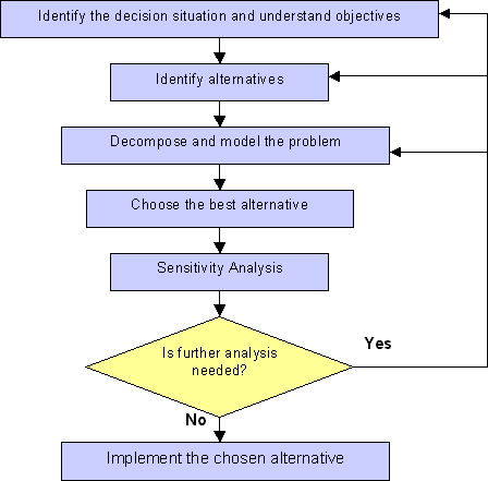
This Web site presents the decision analysis process both for public and private decision making under different decision criteria, type, and quality of available information. This Web site describes the basic elements in the analysis of decision alternatives and choice, as well as the goals and objectives that guide decision making. In the subsequent sections, we will examine key issues related to a decision-maker’s preferences regarding alternatives, criteria for choice, and choice modes.

Objectives are important both in identifying problems and in evaluating alternative solutions. Evaluating alternatives requires that a decision-maker’s objectives be expressed as criterion that reflects the attributes of the alternatives relevant to the choice.

The systematic study of decision making provides a framework for choosing courses of action in a complex, uncertain, or conflict-ridden situation. The choices of possible actions, and the prediction of expected outcomes, derive from a logical analysis of the decision situation.

A Possible Drawback in the Decision Analysis Approach: You might have already noticed that the above criteria always result in selection of only one course of action. However, in many decision problems, the decision-maker might wish to consider a combination of some actions. For example, in the Investment problem, the investor might wish to distribute the assets among a mixture of the choices in such a way to optimize the portfolio's return. Visit the Game Theory with Applications Web site for designing such an optimal mixed strategy.

Further Readings:
Arsham H., A Markovian model of consumer buying behavior and optimal advertising pulsing policy, Computers and Operations Research, 20(2), 35-48, 1993.
Arsham H., A stochastic model of optimal advertising pulsing policy, Computers and Operations Research, 14(3), 231-239, 1987.
Ben-Haim Y., Information-gap Decision Theory: Decisions Under Severe Uncertainty, Academic Press, 2001.
Golub A., Decision Analysis: An Integrated Approach, Wiley, 1997.
Goodwin P., and G. Wright, Decision Analysis for Management Judgment, Wiley, 1998.
van Gigch J., Metadecisions: Rehabilitating Epistemology, Kluwer Academic Publishers, 2002.
Wickham Ph., Strategic Entrepreneurship: A Decision-making Approach to New Venture Creation and Management, Pitman, 1998.


Probabilistic Modeling: From Data to a Decisive Knowledge

Knowledge is what we know well. Information is the communication of knowledge. In every knowledge exchange, there is a sender and a receiver. The sender make common what is private, does the informing, the communicating. Information can be classified as explicit and tacit forms. The explicit information can be explained in structured form, while tacit information is inconsistent and fuzzy to explain. Know that data are only crude information and not knowledge by themselves.

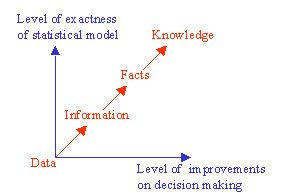
Data is known to be crude information and not knowledge by itself. The sequence from data to knowledge is: from Data to Information, from Information to Facts, and finally, from Facts to Knowledge. Data becomes information, when it becomes relevant to your decision problem. Information becomes fact, when the data can support it. Facts are what the data reveals. However the decisive instrumental (i.e., applied) knowledge is expressed together with some statistical degree of confidence.

Fact becomes knowledge, when it is used in the successful completion of a decision process. Once you have a massive amount of facts integrated as knowledge, then your mind will be superhuman in the same sense that mankind with writing is superhuman compared to mankind before writing. The following figure illustrates the statistical thinking process based on data in constructing statistical models for decision making under uncertainties.
From Data to Knowledge

The above figure depicts the fact that as the exactness of a statistical model increases, the level of improvements in decision-making increases. That's why we need probabilistic modeling. Probabilistic modeling arose from the need to place knowledge on a systematic evidence base. This required a study of the laws of probability, the development of measures of data properties and relationships, and so on.

Statistical inference aims at determining whether any statistical significance can be attached that results after due allowance is made for any random variation as a source of error. Intelligent and critical inferences cannot be made by those who do not understand the purpose, the conditions, and applicability of the various techniques for judging significance.

Knowledge is more than knowing something technical. Knowledge needs wisdom. Wisdom is the power to put our time and our knowledge to the proper use. Wisdom comes with age and experience. Wisdom is the accurate application of accurate knowledge and its key component is to knowing the limits of your knowledge. Wisdom is about knowing how something technical can be best used to meet the needs of the decision-maker. Wisdom, for example, creates statistical software that is useful, rather than technically brilliant. For example, ever since the Web entered the popular consciousness, observers have noted that it puts information at your fingertips but tends to keep wisdom out of reach.

Considering the uncertain environment, the chance that "good decisions" are made increases with the availability of "good information." The chance that "good information" is available increases with the level of structuring the process of Knowledge Management. One may ask, "What is the use of decision analysis techniques without the best available information delivered by Knowledge Management?" The answer is: one can not make responsible decisions until one possess enough knowledge. However, for private decisions one may rely on, e.g., the psychological motivations, as discusses under "Decision Making Under Pure Uncertainty" in this site. Moreover, Knowledge Management and Decision Analysis are indeed interrelated since one influences the other, both in time, and space. The notion of "wisdom" in the sense of practical wisdom has entered Western civilization through biblical texts. In the Hellenic experience this kind of wisdom received a more structural character in the form of philosophy. In this sense philosophy also reflects one of the expressions of traditional wisdom.

Making decisions is certainly the most important task of a manager and it is often a very difficult one. This site offers a decision making procedure for solving complex problems step by step.

The Decision-Making Process: Unlike the deterministic decision-making process, in the decision making process under uncertainty the variables are often more numerous and more difficult to measure and control. However, the steps are the same. They are:

  1. Simplification
  2. Building a decision model
  3. Testing the model
  4. Using the model to find the solution
    • It is a simplified representation of the actual situation
    • It need not be complete or exact in all respects
    • It concentrates on the most essential relationships and ignores the less essential ones.
    • It is more easily understood than the empirical situation and, hence, permits the problem to be more readily solved with minimum time and effort.
  5. It can be used again and again for like problems or can be modified.

Fortunately the probabilistic and statistical methods for analysis and decision making under uncertainty are more numerous and powerful today than even before. The computer makes possible many practical applications. A few examples of business applications are the following:

Further Readings:
Berger J., Statistical Decision Theory and Bayesian Analysis, Springer, 1978.
Corfield D., and J. Williamson, Foundations of Bayesianism, Kluwer Academic Publishers, 2001. Contains Logic, Mathematics, Decision Theory, and Criticisms of Bayesianism.
Grünig R., Kühn, R.,and M. Matt, (Eds.), Successful Decision-Making: A Systematic Approach to Complex Problems, Springer, 2005. It is intended for decision makers in companies, in non-profit organizations and in public administration.
Lapin L., Statistics for Modern Business Decisions, Harcourt Brace Jovanovich, 1987.
Lindley D., Making Decisions, Wiley, 1991.
Pratt J., H. Raiffa, and R. Schlaifer, Introduction to Statistical Decision Theory, The MIT Press, 1994.
Press S., and J. Tanur, The Subjectivity of Scientists and the Bayesian Approach, Wiley, 2001. Comparing and contrasting the reality of subjectivity in the work of history's great scientists and the modern Bayesian approach to statistical analysis.
Tanaka H., and P. Guo, Possibilistic Data Analysis for Operations Research, Physica-Verlag, 1999.


Decision Analysis: Making Justifiable, Defensible Decisions

Decision analysis is the discipline of evaluating complex alternatives in terms of values and uncertainty. Values are generally expressed monetarily because this is a major concern for management. Furthermore, decision analysis provides insight into how the defined alternatives differ from one another and then generates suggestions for new and improved alternatives. Numbers quantify subjective values and uncertainties, which enable us to understand the decision situation. These numerical results then must be translated back into words in order to generate qualitative insight.

Humans can understand, compare, and manipulate numbers. Therefore, in order to create a decision analysis model, it is necessary to create the model structure and assign probabilities and values to fill the model for computation. This includes the values for probabilities, the value functions for evaluating alternatives, the value weights for measuring the trade-off objectives, and the risk preference.

Once the structure and numbers are in place, the analysis can begin. Decision analysis involves much more than computing the expected utility of each alternative. If we stopped there, decision makers would not gain much insight. We have to examine the sensitivity of the outcomes, weighted utility for key probabilities, and the weight and risk preference parameters. As part of the sensitivity analysis, we can calculate the value of perfect information for uncertainties that have been carefully modeled.

There are two additional quantitative comparisons. The first is the direct comparison of the weighted utility for two alternatives on all of the objectives. The second is the comparison of all of the alternatives on any two selected objectives which shows the Pareto optimality for those two objectives.

Complexity in the modern world, along with information quantity, uncertainty, and risk, make it necessary to provide a rational decision making framework. The goal of decision analysis is to give guidance, information, insight, and structure to the decision-making process in order to make better, more 'rational' decisions.

A decision needs a decision maker who is responsible for making decisions. This decision maker has a number of alternatives and must choose one of them. The objective of the decision-maker is to choose the best alternative. When this decision has been made, events that the decision-maker has no control over may have occurred. Each combination of alternatives, followed by an event happening, leads to an outcome with some measurable value. Managers make decisions in complex situations. Decision tree and payoff matrices illustrate these situations and add structure to the decision problems.

Further Readings:
Arsham H., Decision analysis: Making justifiable, defensible decisions, e-Quality, September, 2004.
Forman E., and M. Selly, Decision by Objectives: How to Convince Others That You Are Right, World Scientific, 2001.
Gigerenzer G., Adaptive Thinking: Rationality in the Real World, Oxford University Press, 2000.
Girón F., (Ed.), Applied Decision Analysis, Kluwer Academic, 1998.
Manning N., et al., Strategic Decision Making In Cabinet Government: Institutional Underpinnings and Obstacles, World Bank, 1999.
Patz A., Strategic Decision Analysis: A General Management Framework, Little and Brown Pub., 1981.
Vickers G., The Art of Judgment: A Study of Policy Making, Sage Publications, 1995.
Von Furstenberg G., Acting Under Uncertainty: Multidisciplinary Conceptions, Kluwer Academic Publishers, 1990.


Elements of Decision Analysis Models

The mathematical models and techniques considered in decision analysis are concerned with prescriptive theories of choice (action). This answers the question of exactly how a decision maker should behave when faced with a choice between those actions which have outcomes governed by chance, or the actions of competitors.

Decision analysis is a process that allows the decision maker to select at least and at most one option from a set of possible decision alternatives. There must be uncertainty regarding the future along with the objective of optimizing the resulting payoff (return) in terms of some numerical decision criterion.

The elements of decision analysis problems are as follow:

  1. A sole individual is designated as the decision-maker. For example, the CEO of a company, who is accountable to the shareholders.
  2. A finite number of possible (future) events called the 'States of Nature' (a set of possible scenarios). They are the circumstances under which a decision is made. The states of nature are identified and grouped in set "S"; its members are denoted by "s(j)". Set S is a collection of mutually exclusive events meaning that only one state of nature will occur.
  3. A finite number of possible decision alternatives (i.e., actions) is available to the decision-maker. Only one action may be taken. What can I do? A good decision requires seeking a better set of alternatives than those that are initially presented or traditionally accepted. Be brief on the logic and reason portion of your decision. While there are probably a thousand facts about an automobile, you do not need them all to make a decision. About a half dozen will do.
  4. Payoff is the return of a decision. Different combinations of decisions and states of nature (uncertainty) generate different payoffs. Payoffs are usually shown in tables. In decision analysis payoff is represented by positive (+) value for net revenue, income, or profit and negative (-) value for expense, cost or net loss. Payoff table analysis determines the decision alternatives using different criteria. Rows and columns are assigned possible decision alternatives and possible states of nature, respectively.
    Constructing such a matrix is usually not an easy task; therefore, it may take some practice.

Source of Errors in Decision Making: The main sources of errors in risky decision-making problems are: false assumptions, not having an accurate estimation of the probabilities, relying on expectations, difficulties in measuring the utility function, and forecast errors.
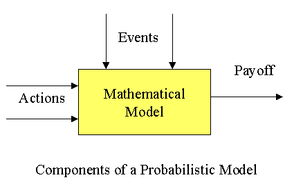
Consider the following Investment Decision-Making Example:

The Investment Decision-Making Example:

States of Nature
Growth Medium G No Change Low
G MG NC L
Bonds 12% 8 7 3
Actions Stocks 15 9 5 -2
Deposit 7 7 7 7

The States of Nature are the states of economy during one year. The problem is to decide what action to take among three possible courses of action with the given rates of return as shown in the body of the table.

Further Readings:
Borden T., and W. Banta, (Ed.), Using Performance Indicators to Guide Strategic Decision Making, Jossey-Bass Pub., 1994.
Eilon S., The Art of Reckoning: Analysis of Performance Criteria, Academic Press, 1984.
Von Furstenberg G., Acting Under Uncertainty: Multidisciplinary Conceptions, Kluwer Academic Publishers, 1990.


Coping With Uncertainties

There are a few satisfactory description of uncertainty, one of which is the concept and the algebra of probability.

To make serious business decisions one is to face a future in which ignorance and uncertainty increasingly overpower knowledge, as ones planning horizon recedes into the distance. The deficiencies about our knowledge of the future may be divided into three domains, each with rather murky boundaries:

While making business decisions, we are largely concerned with the domain of risk and usually assume that the probabilities follow normal distributions. However, we must be concerned with all three domains and have an open mind about the shape of the distributions.

Continuum of pure uncertainty and certainty: The domain of decision analysis models falls between two extreme cases. This depends upon the degree of knowledge we have about the outcome of our actions, as shown below:
Ignorance Risky Situation Complete Knowledge
_______________________________________________________________
Pure Uncertainty Probabilistic Deterministic
Model Model Model

One "pole" on this scale is deterministic, such as the carpenter's problem. The opposite "pole" is pure uncertainty. Between these two extremes are problems under risk. The main idea here is that for any given problem, the degree of certainty varies among managers depending upon how much knowledge each one has about the same problem. This reflects the recommendation of a different solution by each person.

Probability is an instrument used to measure the likelihood of occurrence for an event. When you use probability to express your uncertainty, the deterministic side has a probability of 1 (or zero), while the other end has a flat (all equally probable) probability. For example, if you are certain of the occurrence (or non-occurrence) of an event, you use the probability of one (or zero). If you are uncertain, and would use the expression "I really don't know," the event may or may not occur with a probability of 50%. This is the Bayesian notion that probability assessment is always subjective. That is, the probability always depends upon how much the decision maker knows. If someone knows all there is to know, then the probability will diverge either to 1 or 0.

The decision situations with flat uncertainty have the largest risk. For simplicity, consider a case where there are only two outcomes, with one having a probability of p. Thus, the variation in the states of nature is p(1-p). The largest variation occurs if we set p = 50%, given each outcome an equal chance. In such a case, the quality of information is at its lowest level. Remember from your Statistics course that the quality of information and variation are inversely related. That is, larger variation in data implies lower quality data (i.e. information).

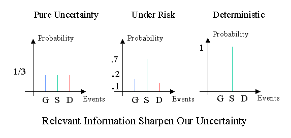
Relevant information and knowledge used to solve a decision problem sharpens our flat probability. Useful information moves the location of a problem from the pure uncertain "pole" towards the deterministic "pole".

Probability assessment is nothing more than the quantification of uncertainty. In other words, quantification of uncertainty allows for the communication of uncertainty between persons. There can be uncertainties regarding events, states of the world, beliefs, and so on. Probability is the tool for both communicating uncertainty and managing it (taming chance).

There are different types of decision models that help to analyze the different scenarios. Depending on the amount and degree of knowledge we have, the three most widely used types are:

In decision-making under pure uncertainty, the decision maker has absolutely no knowledge, not even about the likelihood of occurrence for any state of nature. In such situations, the decision-maker's behavior is purely based on his/her attitude toward the unknown. Some of these behaviors are optimistic, pessimistic, and least regret, among others. The most optimistic person I ever met was undoubtedly a young artist in Paris who, without a franc in his pocket, went into a swanky restaurant and ate dozens of oysters in hopes of finding a pearl to pay the bill.

Optimist: The glass is half-full.
Pessimist: The glass is half-empty.
Manager: The glass is twice as large as it needs to be.

Or, as in the follwoing metaphor of a captain in a rough sea:

The pessimist complains about the wind;
the optimist expects it to change;
the realist adjusts the sails.

Optimists are right; so are the pessimists. It is up to you to choose which you will be. The optimist sees opportunity in every problem; the pessimist sees problem in every opportunity.

Both optimists and pessimists contribute to our society. The optimist invents the airplane and the pessimist the parachute.

Whenever the decision maker has some knowledge regarding the states of nature, he/she may be able to assign subjective probability for the occurrence of each state of nature. By doing so, the problem is then classified as decision making under risk.

In many cases, the decision-maker may need an expert's judgment to sharpen his/her uncertainties with respect to the likelihood of each state of nature. In such a case, the decision-maker may buy the expert's relevant knowledge in order to make a better decision. The procedure used to incorporate the expert's advice with the decision maker's probabilities assessment is known as the Bayesian approach.

For example, in an investment decision-making situation, one is faced with the following question: What will the state of the economy be next year? Suppose we limit the possibilities to Growth (G), Same (S), or Decline (D). Then, a typical representation of our uncertainty could be depicted as follows:

Further Readings:
Howson C., and P. Urbach, Scientific Reasoning: The Bayesian Approach, Open Court Publ., Chicago, 1993.
Gheorghe A., Decision Processes in Dynamic Probabilistic Systems, Kluwer Academic, 1990.
Kouvelis P., and G. Yu, Robust Discrete Optimization and its Applications, Kluwer Academic Publishers, 1997. Provides a comprehensive discussion of motivation for sources of uncertainty in decision process, and a good discussion on minmax regret and its advantages over other criteria.


Decision Making Under Pure Uncertainty

In decision making under pure uncertainty, the decision-maker has no knowledge regarding any of the states of nature outcomes, and/or it is costly to obtain the needed information. In such cases, the decision making depends merely on the decision-maker's personality type.


Personality Types and Decision Making:

Pessimism, or Conservative (MaxMin). Worse case scenario. Bad things always happen to me.
B 3
a) Write min # in each action row, S -2
b) Choose max # and do that action. D 7 *

Optimism, or Aggressive (MaxMax). Good things always happen to me.

B 12
a) Write max # in each action row, S 15 *
b) Choose max # and do that action. D 7

Coefficient of Optimism (Hurwicz's Index), Middle of the road: I am neither too optimistic nor too pessimistic.

a) Choose an a between 0 & 1, 1 means optimistic and 0 means pessimistic,

b) Choose largest and smallest # for each action,

c) Multiply largest payoff (row-wise) by a and the smallest by (1- a ),

d) Pick action with largest sum.

For example, for a = 0.7, we have

B (.7*12) + (.3*3) = 9.3
S (.7*15) + .3*(-2) = 9.9 *
D (.7*7) + (.3*7) = 7

Minimize Regret: (Savag's Opportunity Loss) I hate regrets and therefore I have to minimize my regrets. My decision should be made so that it is worth repeating. I should only do those things that I feel I could happily repeat. This reduces the chance that the outcome will make me feel regretful, or disappointed, or that it will be an unpleasant surprise.

Regret is the payoff on what would have been the best decision in the circumstances minus the payoff for the actual decision in the circumstances. Therefore, the first step is to setup the regret table:


a) Take the largest number in each states of nature column (say, L).
b) Subtract all the numbers in that state of nature column from it (i.e. L - Xi,j).
c) Choose maximum number of each action.
d) Choose minimum number from step (d) and take that action.

The Regret Matrix
G MG NC L
Bonds (15-12) (9-8) (7-7) (7-3) 4 *
Stocks (15-15) (9-9) (7-5) (7+2) 9
Deposit (15-7) (9-7) (7-7) (7-7) 8


You may try checking your computations using Decision Making Under Pure Uncertainty JavaScript, and then performing some numerical experimentation for a deeper understanding of the concepts.

Limitations of Decision Making under Pure Uncertainty

  1. Decision analysis in general assumes that the decision-maker faces a decision problem where he or she must choose at least and at most one option from a set of options. In some cases this limitation can be overcome by formulating the decision making under uncertainty as a zero-sum two-person game.

  2. In decision making under pure uncertainty, the decision-maker has no knowledge regarding which state of nature is "most likely" to happen. He or she is probabilistically ignorant concerning the state of nature therefore he or she cannot be optimistic or pessimistic. In such a case, the decision-maker invokes consideration of security.

  3. Notice that any technique used in decision making under pure uncertainties, is appropriate only for the private life decisions. Moreover, the public person (i.e., you, the manager) has to have some knowledge of the state of nature in order to predict the probabilities of the various states of nature. Otherwise, the decision-maker is not capable of making a reasonable and defensible decision.

You might try to use Decision Making Under Uncertainty JavaScript E-lab for checking your computation, performing numerical experimentation for a deeper understanding, and stability analysis of your decision by altering the problem's parameters.

Further Readings:
Biswas T., Decision Making Under Uncertainty, St. Martin's Press, 1997.
Driver M., K. Brousseau, and Ph. Hunsaker, The Dynamic Decisionmaker: Five Decision Styles for Executive and Business Success, Harper & Row, 1990.
Eiser J., Attitudes and Decisions, Routledge, 1988.
Flin R., et al., (Ed.), Decision Making Under Stress: Emerging Themes and Applications, Ashgate Pub., 1997.
Ghemawat P., Commitment: The Dynamic of Strategy, Maxwell Macmillan Int., 1991.
Goodwin P., and G. Wright, Decision Analysis for Management Judgment, Wiley, 1998.


Decision Making Under Risk

Risk implies a degree of uncertainty and an inability to fully control the outcomes or consequences of such an action. Risk or the elimination of risk is an effort that managers employ. However, in some instances the elimination of one risk may increase some other risks. Effective handling of a risk requires its assessment and its subsequent impact on the decision process. The decision process allows the decision-maker to evaluate alternative strategies prior to making any decision. The process is as follows:

  1. The problem is defined and all feasible alternatives are considered. The possible outcomes for each alternative are evaluated.
  2. Outcomes are discussed based on their monetary payoffs or net gain in reference to assets or time.
  3. Various uncertainties are quantified in terms of probabilities.
  4. The quality of the optimal strategy depends upon the quality of the judgments. The decision-maker should identify and examine the sensitivity of the optimal strategy with respect to the crucial factors.

Whenever the decision maker has some knowledge regarding the states of nature, he/she may be able to assign subjective probability estimates for the occurrence of each state. In such cases, the problem is classified as decision making under risk. The decision-maker is able to assign probabilities based on the occurrence of the states of nature. The decision making under risk process is as follows:

a) Use the information you have to assign your beliefs (called subjective probabilities) regarding each state of the nature, p(s),

b) Each action has a payoff associated with each of the states of nature X(a,s),

c) We compute the expected payoff, also called the return (R), for each action R(a) = Sums of [X(a,s) p(s)],

d) We accept the principle that we should minimize (or maximize) the expected payoff,

e) Execute the action which minimizes (or maximize) R(a).


Expected Payoff: The actual outcome will not equal the expected value. What you get is not what you expect, i.e. the "Great Expectations!"

a) For each action, multiply the probability and payoff and then,
b) Add up the results by row,
c) Choose largest number and take that action.

G (0.4) MG (0.3) NC (0.2) L (0.1) Exp. Value
B 0.4(12) + 0.3(8) + 0.2(7) + 0.1(3) = 8.9
S 0.4(15) + 0.3(9) + 0.2(5) + 0.1(-2) = 9.5*
D 0.4(7) + 0.3(7) + 0.2(7) + 0.1(7) = 7


The Most Probable States of Nature (good for non-repetitive decisions)

a) Take the state of nature with the highest probability (subjectively break any ties),
b) In that column, choose action with greatest payoff.

In our numerical example, there is a 40% chance of growth so we must buy stocks.

Expected Opportunity Loss (EOL):

a) Setup a loss payoff matrix by taking largest number in each state of nature column(say L), and subtract all numbers in that column from it, L - Xij,
b) For each action, multiply the probability and loss then add up for each action,
c) Choose the action with smallest EOL.

Loss Payoff Matrix
G (0.4) MG (0.3) NC (0.2) L (0.1) EOL
B 0.4(15-12) + 0.3(9-8) + 0.2(7-7) + 0.1(7-3) 1.9
S 0.4(15-15) + 0.3(9-9) + 0.2(7-5) + 0.1(7+2) 1.3*
D 0.4(15-7) + 0.3(9-7) + 0.2(7-7) + 0.1(7-7) 3.8

Computation of the Expected Value of Perfect Information (EVPI)

EVPI helps to determine the worth of an insider who possesses perfect information. Recall that EVPI = EOL.

a) Take the maximum payoff for each state of nature,
b) Multiply each case by the probability for that state of nature and then add them up,
c) Subtract the expected payoff from the number obtained in step (b)


G 15(0.4) = 6.0
MG 9(0.3) = 2.7
NC 7(0.2) = 1.4
L 7(0.1) = 0.7
+ ----------
10.8

Therefore, EVPI = 10.8 - Expected Payoff = 10.8 - 9.5 = 1.3. Verify that EOL=EVPI.

The efficiency of the perfect information is defined as 100 [EVPI/(Expected Payoff)]%

Therefore, if the information costs more than 1.3% of investment, don't buy it. For example, if you are going to invest $100,000, the maximum you should pay for the information is [100,000 * (1.3%)] = $1,300

I Know Nothing: (the Laplace equal likelihood principle) Every state of nature has an equal likelihood. Since I don't know anything about the nature, every state of nature is equally likely to occur:

a) For each state of nature, use an equal probability (i.e., a Flat Probability),
b) Multiply each number by the probability,
c) Add action rows and put the sum in the Expected Payoff column,
d) Choose largest number in step (c) and perform that action.

G MG NC L Exp. Payoff
Bonds 0.25(12) 0.25(8) 0.25(7) 0.25(3) 7.5 *
Stocks 0.25(15) 0.25(9) 0.25(5) 0.25(-2) 6.75
Deposit 0.25(7) 0.25(7) 0.25(7) 0.25(7) 7

A Discussion on Expected Opportunity Loss (Expected Regret): Comparing a decision outcome to its alternatives appears to be an important component of decision-making. One important factor is the emotion of regret. This occurs when a decision outcome is compared to the outcome that would have taken place had a different decision been made. This is in contrast to disappointment, which results from comparing one outcome to another as a result of the same decision. Accordingly, large contrasts with counterfactual results have a disproportionate influence on decision making.

Regret results compare a decision outcome with what might have been. Therefore, it depends upon the feedback available to decision makers as to which outcome the alternative option would have yielded. Altering the potential for regret by manipulating uncertainty resolution reveals that the decision-making behavior that appears to be risk averse can actually be attributed to regret aversion.

There is some indication that regret may be related to the distinction between acts and omissions. Some studies have found that regret is more intense following an action, than an omission. For example, in one study, participants concluded that a decision maker who switched stock funds from one company to another and lost money, would feel more regret than another decision maker who decided against switching the stock funds but also lost money. People usually assigned a higher value to an inferior outcome when it resulted from an act rather than from an omission. Presumably, this is as a way of counteracting the regret that could have resulted from the act.

You might like to use Making Risky Decisions JavaScript E-lab for checking your computation, performing numerical experimentation for a deeper understanding, and stability analysis of your decision by altering the problem's parameters.

Further Readings:
Beroggi G., Decision Modeling in Policy Management: An Introduction to the Analytic Concepts, Boston, Kluwer Academic Publishers, 1999.
George Ch., Decision Making Under Uncertainty: An Applied Statistics Approach, Praeger Pub., 1991.
Rowe W., An Anatomy of Risk, R.E. Krieger Pub. Co., 1988.
Suijs J., Cooperative Decision-Making Under Risk, Kluwer Academic, 1999.


Making a Better Decision by Buying Reliable Information (Bayesian Approach)

In many cases, the decision-maker may need an expert's judgment to sharpen his/her uncertainties with respect to the probable likelihood of each state of nature. For example, consider the following decision problem a company is facing concerning the development of a new product:


States of Nature
High Sales Med. Sales Low Sales
A(0.2) B(0.5) C(0.3)
A1 (develop) 3000 2000 -6000
A2 (don't develop) 0 0 0

The probabilities of the states of nature represent the decision-maker's (e.g. manager) degree of uncertainties and personal judgment on the occurrence of each state. We will refer to these subjective probability assessments as 'prior' probabilities.

The expected payoff for each action is:

A1= 0.2(3000) + 0.5(2000) + 0.3(-6000)= $ -200 and A2= 0;

so the company chooses A2 because of the expected loss associated with A1, and decides not to develop.

However, the manager is hesitant about this decision. Based on "nothing ventured, nothing gained" the company is thinking about seeking help from a marketing research firm. The marketing research firm will assess the size of the product's market by means of a survey.

Now the manager is faced with a new decision to make; which marketing research company should he/she consult? The manager has to make a decision as to how 'reliable' the consulting firm is. By sampling and then reviewing the past performance of the consultant, we can develop the following reliability matrix:

1. Given What Actually Happened in the Past
A B C
2. What the Ap 0.8 0.1 0.1
Consultant Bp 0.1 0.9 0.2
Predicted Cp 0.1 0.0 0.7

All marketing research firms keep records (i.e., historical data) of the performance of their past predictions. These records are available to their clients free of charge. To construct a reliability matrix, you must consider the marketing research firm's performance records for similar products with high sales. Then, find the percentage of which products the marketing research firm correctly predicted would have high sales (A), medium sales (B), and little (C) or almost no sales. Their percentages are presented by
P(Ap|A) = 0.8, P(Bp|A) = 0.1, P(Cp|A) = 0.1,
in the first column of the above table, respectively. Similar analysis should be conducted to construct the remaining columns of the reliability matrix.

Note that for consistency, the entries in each column of the above reliability matrix should add up to one. While this matrix provides the conditional probabilities such as P(Ap|A) = 0.8, the important information the company needs is the reverse form of these conditional probabilities. In this example, what is the numerical value of P(A|Ap)? That is, what is the chance that the marketing firm predicts A is going to happen, and A actually will happen? This important information can be obtained by applying the Bayes Law (from your probability and statistics course) as follows:

a) Take probabilities and multiply them "down" in the above matrix,
b) Add the rows across to get the sum,
c) Normalize the values (i.e. making probabilities adding up to 1) by dividing each column number by the sum of the row found in Step b,

0.2 0.5 0.3
A B C SUM
02(0.8) = 0.16 0.5(0.1) = 0.05 0.3(0.1) = 0.03 0.24
0.2(0.1) = 0.02 0.5(0.9) = 0.45 0.3(0.2) = 0.06 0.53
0.2(0.1) = 0.02 0.5(0) = 0 0.3(0.7) = 0.21 0.23

A B C
(.16/.24)=.667 (.05/.24)=.208 (.03/.24)=.125
(.02/.53)=.038 (0.45/.53)=.849 (.06/.53)=.113
(.02/.23)=.087 (0/.23)=0 (0.21/.23)=.913

You might like to use Computational Aspect of Bayse' Revised Probability JavaScript E-lab for checking your computation, performing numerical experimentation for a deeper understanding, and stability analysis of your decision by altering the problem's parameters.

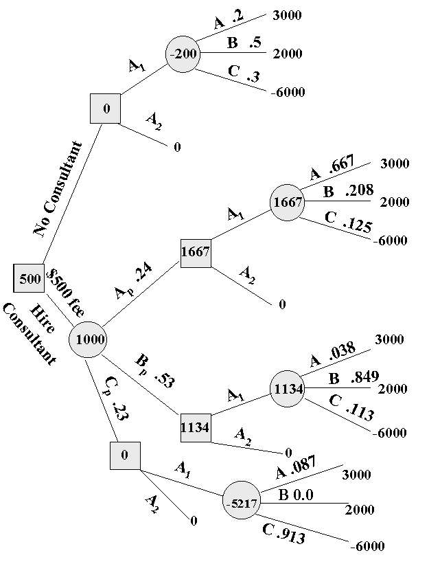
d) Draw the decision tree. Many managerial problems, such as this example, involve a sequence of decisions. When a decision situation requires a series of decisions, the payoff table cannot accommodate the multiple layers of decision-making. Thus, a decision tree is needed.

Do not gather useless information that cannot change a decision: A question for you: In a game a player is presented two envelopes containing money. He is told that one envelope contains twice as much money as the other envelope, but he does not know which one contains the larger amount. The player then may pick one envelope at will, and after he has made a decision, he is offered to exchange his envelope with the other envelope.
If the player is allowed to see what's inside the envelope he has selected at first, should the player swap, that is, exchange the envelopes?
The outcome of a good decision may not be good, therefor one must not confuse the quality of the outcome with the quality of the decision.
As Seneca put it "When the words are clear, then the thought will be also".


Decision Tree and Influence Diagram

Decision Tree Approach: A decision tree is a chronological representation of the decision process. It utilizes a network of two types of nodes: decision (choice) nodes (represented by square shapes), and states of nature (chance) nodes (represented by circles). Construct a decision tree utilizing the logic of the problem. For the chance nodes, ensure that the probabilities along any outgoing branch sum to one. Calculate the expected payoffs by rolling the tree backward (i.e., starting at the right and working toward the left).

You may imagine driving your car; starting at the foot of the decision tree and moving to the right along the branches. At each square you have control, to make a decision and then turn the wheel of your car. At each circle, Lady Fortuna takes over the wheel and you are powerless.

Here is a step-by-step description of how to build a decision tree:

  1. Draw the decision tree using squares to represent decisions and circles to represent uncertainty,
  2. Evaluate the decision tree to make sure all possible outcomes are included,
  3. Calculate the tree values working from the right side back to the left,
  4. Calculate the values of uncertain outcome nodes by multiplying the value of the outcomes by their probability (i.e., expected values).

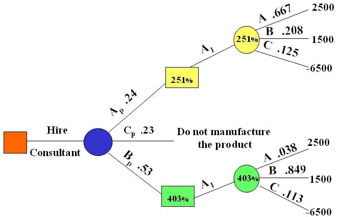
On the tree, the value of a node can be calculated when we have the values for all the nodes following it. The value for a choice node is the largest value of all nodes immediately following it. The value of a chance node is the expected value of the nodes following that node, using the probability of the arcs. By rolling the tree backward, from its branches toward its root, you can compute the value of all nodes including the root of the tree. Putting these numerical results on the decision tree results in the following graph:

A Typical Decision Tree
Click on the image to enlarge it

Determine the best decision for the tree by starting at its root and going forward.

Based on proceeding decision tree, our decision is as follows:

Hire the consultant, and then wait for the consultant's report.
If the report predicts either high or medium sales, then go ahead and manufacture the product.
Otherwise, do not manufacture the product.

Check the consultant's efficiency rate by computing the following ratio:

(Expected payoff using consultant dollars amount) / EVPI.

Using the decision tree, the expected payoff if we hire the consultant is:

EP = 1000 - 500 = 500,

EVPI = .2(3000) + .5(2000) + .3(0) = 1600.

Therefore, the efficiency of this consultant is: 500/1600 = 31%

If the manager wishes to rely solely on the marketing research firm's recommendations, then we assign flat prior probability [as opposed to (0.2, 0.5, 0.3) used in our numerical example].

Clearly the manufacturer is concerned with measuring the risk of the above decision, based on decision tree.

Coefficient of Variation as Risk Measuring Tool and Decision Procedure: Based on the above decision, and its decision-tree, one might develop a coefficient of variation (C.V) risk-tree, as depicted below:

Coefficient of Variation as a Risk Measuring Tool and Decision Procedure
Click on the image to enlarge it

Notice that the above risk-tree is extracted from the decision tree, with C.V. numerical value at the nodes relevant to the recommended decision. For example the consultant fee is already subtracted from the payoffs.

From the above risk-tree, we notice that this consulting firm is likely (with probability 0.53) to recommend Bp (a medium sales), and if you decide to manufacture the product then the resulting coefficient of variation is very high (403%), compared with the other branch of the tree (i.e., 251%).

Clearly one must not consider only one consulting firm, rather one must consider several potential consulting during decision-making planning stage. The risk decision tree then is a necessary tool to construct for each consulting firm in order to measure and compare to arrive at the final decision for implementation.

The Impact of Prior Probability and Reliability Matrix on Your Decision: To study how important your prior knowledge and/or the accuracy of the expected information from the consultant in your decision our numerical example, I suggest redoing the above numerical example in performing some numerical sensitivity analysis. You may start with the following extreme and interesting cases by using this JavaScript for the needed computation:

Influence diagrams: As can be seen in the decision tree examples, the branch and node description of sequential decision problems often become very complicated. At times it is downright difficult to draw the tree in such a manner that preserves the relationships that actually drive the decision. The need to maintain validation, and the rapid increase in complexity that often arises from the liberal use of recursive structures, have rendered the decision process difficult to describe to others. The reason for this complexity is that the actual computational mechanism used to analyze the tree, is embodied directly within the trees and branches. The probabilities and values required to calculate the expected value of the following branch are explicitly defined at each node.

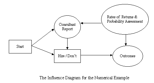
Influence diagrams are also used for the development of decision models and as an alternate graphical representations of decision trees. The following figure depicts an influence diagram for our numerical example.


In the influence diagram above, the decision nodes and chance nodes are similarly illustrated with squares and circles. Arcs (arrows) imply relationships, including probabilistic ones.

Finally, decision tree and influence diagram provide effective methods of decision-making because they:

Visit also:
Decision Theory and Decision Trees

Further Readings
Bazerman M., Judgment in Managerial Decision Making, Wiley, 1993.
Connolly T., H. Arkes, and K. Hammond (eds), Judgment and Decision Making: An Interdisciplinary Reader, Cambridge University Press, 2000.
Cooke R., Experts in Uncertainty, Oxford Univ Press, 1991. Describes much of the history of the expert judgment problem. It also includes many of the methods that have been suggested to do numerical combination of expert uncertainties. Furthermore, it promotes a method that has been used extensively by us and many others, in which experts are given a weighting that judge their performance on calibration questions. This is a good way of getting around the problem of assessing the "quality" of an expert, and lends a degree of objectivity to the results that is not obtained by other methods.
Bouyssou D., et al., Evaluation and Decision Models: A Critical Perspective, Kluwer Academic Pub, 2000.
Daellenbach H., Systems and Decision Making: A Management Science Approach, Wiley, 1994.
Goodwin P., and G. Wright, Decision Analysis for Management Judgment, Wiley, 1998.
Klein D., Decision-Analytic Intelligent Systems: Automated Explanation and Knowledge Acquisition, Lawrence Erlbaum Pub., 1994.
Thierauf R., Creative Computer Software for Strategic Thinking and Decision Making: A Guide for Senior Management and MIS Professionals, Quorum Books, 1993.


Why Managers Seek the Advice From Consulting Firms

Managers pay consultants to provide advisory service work that falls into one of the following categories:

  • Work they are not -- or feel they are not — competent to do themselves.

  • Work they do not want to do themselves.

  • Work they do not have time to do themselves.

All such work falls under the broad umbrella of consulting service. Regardless of why managers pay others to advise them, they typically have high expectations concerning the quality of the recommendations, measured in terms of reliability and cost. However, the manager is solely responsible for the final decision he/she is making and not the consultants.

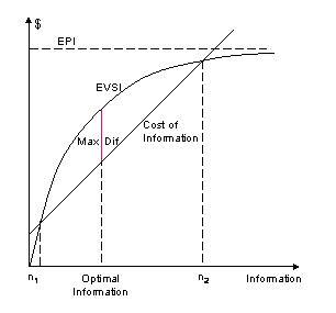
The following figure depicts the process of the optimal information determination. For more details, read the Cost/Benefit Analysis.


The Determination of the Optimal Information


Deciding about the Consulting Firm: Each time you are thinking of hiring a consultant you may face the danger of looking foolish, not to mention losing thousands or even millions of dollars. To make matters worse, most of the consulting industry's tried-and-true firms have recently merged, split, disappeared, reappeared, or reconfigured at least once.

How can you be sure to choose the right consultants?

Test the consultant's knowledge of your product. It is imperative to find out the depth of a prospective consultant's knowledge about your particular product and its potential market. Ask the consultant to provide a generic project plan, task list, or other documentation about your product.

Is there an approved budget and duration?
What potential customers' involvement is expected?
Who is expected to provide the final advice and provide sign-off?

Even the best consultants are likely to have some less-than-successful moments in their work history. Conducting the reliability analysis process is essential. Ask specific questions about the consultants' past projects, proud moments, and failed efforts. Of course it's important to check a potential consultant's references. Ask for specific referrals from as many previous clients or firms with similar businesses to yours. Get a clearly written contract, accurate cost estimates, the survey statistical sample size, and the commitment on the completion and written advice on time.

Further Reading
Holtz H., The Complete Guide to Consulting Contracts: How to Understand, Draft, and Negotiate Contracts and Agreements that Work, Dearborn Trade, 1997.
Weinberg G., Secrets of Consulting: A Guide to Giving and Getting Advice Successfully, Dorset House, 1986.


Revising Your Expectation and its Risk

In our example, we saw how to make decision based on objective payoff matrix by computing the expected value and the risk expressed as coefficient of variation as our decision criteria. While, an informed decision-maker might be able to construct his/her subjective payoff matrix, and then following the same decision process, however, in many situations it becomes necessary to combine the two.

Application: Suppose the following information is available from two independent sources:

Revising the Expected Value and the Variance
Estimate SourceExpected value Variance
Sales manager m1 = 110 s12 = 100
Market survey m2 = 70 s22 = 49

The combined expected value is:

[m1/s12 + m2/s22 ] / [1/s12 + 1/s22]

The combined variance is:

2 / [1/s12 + 1/s22]

For our application, using the above tabular information, the combined estimate of expected sales is 83.15 units with combined variance of 65.77, having 9.6% risk value.

You may like using Revising the Mean and Variance JavaScript to performing some numerical experimentation. You may apply it for validating the above example and for a deeper understanding of the concept where more than 2-sources of information are to be combined.


Determination of the Decision-Maker's Utility Function

We have worked with payoff tables expressed in terms of expected monetary value. Expected monetary value, however, is not always the best criterion to use in decision making. The value of money varies from situation to situation and from one decision maker to another. Generally, too, the value of money is not a linear function of the amount of money. In such situations, the analyst should determine the decision-maker's utility for money and select the alternative course of action that yields the highest expected utility, rather than the highest expected monetary value.

Individuals pay insurance premiums to avoid the possibility of financial loss associated with an undesirable event occurring. However, utilities of different outcomes are not directly proportional to their monetary consequences. If the loss is considered to be relatively large, an individual is more likely to opt to pay an associated premium. If an individual considers the loss inconsequential, it is less likely the individual will choose to pay the associated premium.

Individuals differ in their attitudes towards risk and these differences will influence their choices. Therefore, individuals should make the same decision each time relative to the perceived risk in similar situations. This does not mean that all individuals would assess the same amount of risk to similar situations. Further, due to the financial stability of an individual, two individuals facing the same situation may react differently but still behave rationally. An individual's differences of opinion and interpretation of policies can also produce differences.

The expected monetary reward associated with various decisions may be unreasonable for the following two important reasons:

1. Dollar value may not truly express the personal value of the outcome. This is what motivates some people to play the lottery for $1.

2. Expected monetary values may not accurately reflect risk aversion. For example, suppose you have a choice of between getting $10 dollars for doing nothing, or participating in a gamble. The gamble's outcome depends on the toss of a fair coin. If the coin comes up heads, you get $1000. However, if it is tails, you take a $950 loss.

The first alternative has an expected reward of $10, the second has an expected reward of
0.5(1000) + 0.5(- 950) = $25. Clearly, the second choice is preferred to the first if expected monetary reward were a reasonable criterion. But, you may prefer a sure $10 to running the risk of losing $950.

Why do some people buy insurance and others do not? The decision-making process involves psychological and economical factors, among others. The utility concept is an attempt to measure the usefulness of money for the individual decision maker. It is measured in 'Utile'. The utility concept enables us to explain why, for example, some people buy one dollar lotto tickets to win a million dollars. For these people 1,000,000 ($1) is less than ($1,000,000). These people value the chance to win $1,000,000 more than the value of the $1 to play. Therefore, in order to make a sound decision considering the decision-maker's attitude towards risk, one must translate the monetary payoff matrix into the utility matrix. The main question is: how do we measure the utility function for a specific decision maker?

Consider our Investment Decision Problem. What would the utility of $12 be?

a) Assign 100 utils and zero utils to the largest and smallest ($) payoff, respectively in the payoff matrix. For our numerical example, we assign 100 utils to 15, and 0 utils to -2,

b) Ask the decision maker to choose between the following two scenarios:

1) Get $12 for doing nothing (called, the certainty equivalent, the difference between a decision maker's certainty equivalent and the expected monetary value is called the risk premium.)

OR

2) Play the following game: win $15 with probability (p) OR -$2 with probability (1-p), where p is a selected number between 0 and 1.

By changing the value of p and repeating a similar question, there exists a value for p at which the decision maker is indifferent between the two scenarios. Say, p = 0.58.

c) Now, the utility for $12 is equal to
0.58(100) + (1-0.58)(0) = 58.

d) Repeat the same process to find the utilities for each element of the payoff matrix. Suppose we find the following utility matrix:

Monetary Payoff Matrix Utility Payoff Matrix
A B C D A B C D
12 8 7 3 58 28 20 13
15 9 5 -2 100 30 18 0
7 7 7 7 20 20 20 20

At this point, you may apply any of the previously discussed techniques to this utility matrix (instead of monetary) in order to make a satisfactory decision. Clearly, the decision could be different.

Notice that any technique used in decision making with utility matrix is indeed very subjective; therefore it is more appropriate only for the private life decisions.

You may like to check your computations using Determination of Utility Function JavaScript, and then perform some numerical experimentation for a deeper understanding of the concepts.


Utility Function Representations with Applications

Introduction: A utility function transforms the usefulness of an outcome into a numerical value that measures the personal worth of the outcome. The utility of an outcome may be scaled between 0, and 100, as we did in our numerical example, converting the monetary matrix into the utility matrix . This utility function may be a simple table, a smooth continuously increasing graph, or a mathematical expression of the graph.

The aim is to represent the functional relationship between the entries of monetary matrix and the utility matrix outcome obtained earlier. You may ask what is a function?

What is a function? A function is a thing that does something. For example, a coffee grinding machine is a function that transforms the coffee beans into powder. A utility function translates (converts) the input domain (monetary values) into output range, with the two end-values of 0 and 100 utiles. In other words, a utility function determines the degrees of the decision-maker sensible preferences.

This chapter presents a general process for determining utility function. The presentation is in the context of the previous chapter's numerical results, although there are repeated data therein.

Utility Function Representations with Applications: There are three different methods of representing a function: The Tabular, Graphical, and Mathematical representation. The selection of one method over another depends on the mathematical skill of the decision-maker to understand and use it easily. The three methods are evolutionary in their construction process, respectively; therefore, one may proceed to the next method if needed.

The utility function is often used to predict the utility of the decision-maker for a given monetary value. The prediction scope and precision increases form the tabular method to the mathematical method.

Tabular Representation of the Utility Function: We can tabulate the pair of data (D, U) using the entries of the matrix representing the monetary values (D) and their corresponding utiles (U) from the utility matrix obtained already. The Tabular Form of the utility function for our numerical example is given by the following paired (D, U) table:

Utility Function (U) of the Monetary Variable (D) in Tabular Form

D
12
8
7
3
15
9
5
-2
7
7
7
7
U
58
28
20
13
100
30
18
0
20
20
20
20

Tabular Representation of the Utility Function for the Numerical Example

As you see, the tabular representation is limited to the numerical values within the table. Suppose one wishes to obtain the utility of a dollar value, say $10. One may apply an interpolation method: however since the utility function is almost always non-linear; the interpolated result does not represent the utility of the decision maker accurately. To overcome this difficulty, one may use the graphical method.

Graphical Representation of the Utility Function: We can draw a curve using a scatter diagram obtained by plotting the Tabular Form on a graph paper. Having the scatter diagram, first we need to decide on the shape of the utility function. The utility graph is characterized by its properties of being smooth, continuous, and an increasing curve. Often a parabola shape function fits well for relatively narrow domain values of D variable. For wider domains, one may fit few piece-wise parabola functions, one for each appropriate sub-domain.

For our numerical example, the following is a graph of the function over the interval used in modeling the utility function, plotted with its associated utility (U-axis) and the associated Dollar values (D-axis). Note that in the scatter diagram the multiple points are depicted by small circles.

Graphical Representation of the Utility Function for the Numerical Example

The graphical representation has a big advantage over the tabular representation in that one may read the utility of dollar values say $10, directly from the graph, as shown on the above graph, for our numerical example. The result is U = 40, approximately. Reading a value from a graph is not convenient; therefore, for prediction proposes, a mathematical model serves best.

Mathematical Representation of the Utility Function: We can construct a mathematical model for the utility function using the shape of utility function obtained by its representation by Graphical Method. Often a parabola shape function fits well for relatively narrow domain values of D variable. For wider domains, one may fit a few piece-wise parabola functions, one for each appropriate sub-domain.

We know that we want a quadratic function that best fits the scatter diagram that has already been constructed. Therefore, we use a regression analysis to estimate the coefficients in the function that is the best fit to the pairs of data (D, U).

Parabola models: Parabola regressions have three coefficients with a general form:

U = a + bD + cD2,

where

c = { S (Di - Dbar)2×Ui - n[S(Di - Dbar) 2× SUi]} / {n S(Di - Dbar) 4 - [S(Di - Dbar)2] 2}

b = [S(Di- Dbar) Ui]/[ S(Di - Dbar)2] - 2×c×Dbar

a = {SUi - [c× S(D i - Dbar) 2)}/n - (c×Dbar×Dbar + b×Dbar),

where Dbar is the mean of Di's.

For our numerical example i = 1, 2,..., 12. By evaluating these coefficients using the information given in tabular form section, the "best" fit is characterized by its coefficients estimated values: c = 0.291, b = 1.323, and a = 0.227. The result is; therefore, a utility function approximated by the following quadratic function:

U = 0.291D2 + 1.323D + 0.227,    for all D such that   -2 £ D £ 15.

The above mathematical representation provides more useful information than the other two methods. For example, by taking the derivative of the function provides the marginal value of the utility; i.e.,

Marginal Utility = 1.323 + 0.582D,     for all D such that   -2 < D < 15.

Notice that for this numerical example, the marginal utility is an increasing function, because variable D has a positive coefficient; therefore, one is able to classify this decision- maker as a mild risk-taker.

You might like to use Quadratic Regression JavaScript to check your hand computation. For higher degrees than quadratic, you may like to use the Polynomial Regressions JavaScript.


A Classification of Decision Maker's Relative Attitudes Toward Risk and Its Impact

Probability of an Event and the Impact of its Occurrence: The process-oriented approach of managing the risk and uncertainty is part of any probabilistic modeling. It allows the decision maker to examine the risk within its expected return, and identify the critical issues in assessing, limiting, and mitigating risk. This process involves both the qualitative and quantitative aspects of assessing the impact of risk.

Decision theory does not describe what people actually do since there are difficulties with both computations of probability and the utility of an outcome. Decisions can also be affected by people's subjective rationality and by the way in which a decision problem is perceived.

Traditionally, the expected value of random variables has been used as a major aid to quantify the amount of risk. However, the expected value is not necessarily a good measure alone by which to make decisions since it blurs the distinction between probability and severity. To demonstrate this, consider the following example:

Suppose that a person must make a choice between scenarios 1 and 2 below:

  • Scenario 1: There is a 50% chance of a loss of $50, and a 50% chance of no loss.

  • Scenario 2: There is a 1% chance of a loss of $2,500, and a 99% chance of no loss.

Both scenarios result in an expected loss of $25, but this does not reflect the fact that the second scenario might be considered to be much more risky than the first. (Of course, this is a subjective assessment). The decision maker may be more concerned about minimizing the effect of the occurrence of an extreme event than he/she is concerned about the mean. The following charts depict the complexity of probability of an event and the impact of the occurrence of the event, and its related risk indicator, respectively:

From the previous section, you may recall that the certainty equivalent is the risk free payoff. Moreover, the difference between a decision maker's certainty equivalent and the expected monetary value (EMV) is called the risk premium. We may use the sign and the magnitude of the risk premium in classification of a decision maker's relative attitude toward risk as follows:

  • If the risk premium is positive, then the decision maker is willing to take the risk and the decision maker is said to be a risk seeker. Clearly, some people are more risk-accepting than others: the larger is the risk premium, the more risk-accepting the decision-maker.

  • If the risk premium is negative, then the decision-maker would avoid taking the risk and the decision maker is said to be risk averse.

  • If the risk premium is zero, then the decision maker is said to be risk neutral.

Buying Insurance: As we have noticed, often it is not probability, but expectation that acts a measuring tool and decision-guide. Many decision cases are similar to the following: The probability of a fire in your neighborhood may be very small. But, if it occurred, the cost to you could be very great. Not only property but also your "dear ones", so the negative expectation of not ensuring against fire is so much greater than the cost of premium than ensuring is the best.

Further Readings
Christensen C., The Innovator's Dilemma: When New Technologies Cause Great Firms to Fail, Harvard Business School Publishing, 1997.
Eilon S., The Art of Reckoning: Analysis of Performance Criteria, Academic Press, 1984.
Hammond J., R. Keeney, and H. Raiffa, Smart Choices: A Practical Guide to Making Better Decisions, Harvard Business School Press., 1999.
Richter M., and K. Wong, Computable preference and utility, Journal of Mathematical Economics, 32(3), 339-354, 1999.
Tummala V., Decision Analysis with Business Applications, Educational Publishers, 1973.


The Discovery and Management of Losses

In discovery and management of losses (expressed in the monetary terms) perception and measuring the chance of events is crucial. Losses might have various sources. These sources include Employees, Procedures, and External factors.
  • Employees: Some employees may have concentration problem, insufficient knowledge, and engage in fraud.
  • Procedures: Some procedures are wrongly designed, or they are wrongly implemented.
  • External factors: These include dependency on external unreliable services and suppliers, lack of security form external criminal activities, and finally disasters, such as strong earthquakes.

A rare or unexpected event with potentially significant consequences for decision-making could be conceived as a risk or an opportunity. The main concerns are: How to predict, identify or explain chance events and their consequences? How to assess, prepare for or manage them?

A decision-maker who is engaged in planning, needs to adopt a view for the future, in order to decide goals, and to decide the best sequence of actions to achieve these goals by forecasting their consequences. Unfortunately, the unlikeness of such events makes them difficult to predict or explain by methods that use historical data. However, focusing on the decision-maker's psychological-attitude factors and its environment is mostly relevant.

The following figure provides a classification of the loss frequency function together with the ranges for the Expected, Unexpected, and the Stress, which must be determined by the decision-makers ability and resources.

The manager's ability to discover both unexpected and stress loss events and forecast their consequences is the major task. This is because, these event are very unlikely, therefore making them difficult to predict or explain. However, once a rare event has been identified, the main concern is its consequences for the organization. A good manager cannot ignore these events, as their consequences are significant. For example, although strong earthquakes occur in major urban centers only rarely such earthquakes tend to have human and economic consequences well beyond that of the typical tremor. A rational public safety body for a city in an earthquake-prone area would plan for such contingencies even though the chance of a strong quake is still very small.

Further Readings
Belluck D., and S. Benjamin, A Practical Guide to Understanding, Managing and Reviewing Risk Assessment Reports, CRC Press, 1999.
Koller G., Risk Assessment and Decision Making in Business and Industry: A Practical Guide, CRC Press, 1999.
Hoffman D., Managing Operational Risk: 20 Firmwide Best Practice Strategies, Wiley, 2002
Van Asselt M., Perspectives on Uncertainty and Risk: The Prima Approach to Decision Support, Kluwer Academic Publishers, 2000.


Risk Assessment & Coping Strategies:
How Good Is Your Decision?

Risk is the downside of a gamble, which is described in terms of probability. Risk assessment is a procedure of quantifying the loss or gain values and supplying them with proper values of probabilities. In other words, risk assessment means constructing the random variable that describes the risk. Risk indicator is a quantity describing the quality of the decision.

Considering our earlier Investment Decision-Making Example:

States of Nature
Growth Medium G No Change Low
G MG N L
Bonds 12% 8 7 3
Actions Stocks 15 9 5 -2
Deposit 7 7 7 7

The states of nature are the states of economy during, an arbitrary time frame, as in one year.

The expected value (i.e., the averages) is defined by:

Expected Value = m = SXi . Pi,     the sum is over all i's.

The expected value alone is not a good indication of a quality decision. The variance must be known so that an educated decision may be made. Have you ever heard the dilemma of the six-foot tall statistician who drowned in a stream that had an average depth of three feet?

In the investment example, it is also interesting to compare the 'risk' between alternative courses of action. A measure of risk is generally reported by variation, or its square root called standard deviation. Variation or standard deviation are numerical values that indicate the variability inherent to your decision. For risk, smaller values indicate that what you expect is likely to be what you get. Therefore, risk must also be used when you want to compare alternate courses of action. What we desire is a large expected return, with small risk. Thus, high risk makes a manager very worried.

Variance: An important measure of risk is variance which is defined by:

Variance = s2 = S [Xi2 . Pi] - m2,     the sum is over all i's.

Since the variance is a measure of risk, therefore, the greater the variance, the higher the risk. The variance is not expressed in the same units as the expected value. So, the variance is hard to understand and explain as a result of the squared term in its computation. This can be alleviated by working with the square root of the variance which is called the Standard Deviation:

Standard Deviation = s = (Variance) ½

Both variance and standard deviation provide the same information and, therefore, one can always be obtained from the other. In other words, the process of computing standard deviation always involves computing the variance. Since standard deviation is the square root of the variance, it is always expressed in the same units as the expected value.

For the dynamic decision process, the Volatility as a measure for risk includes the time period over which the standard deviation is computed. The Volatility measure is defined as standard deviation divided by the square root of the time duration.

What should you do if the course of action with the larger expected outcome also has a much higher risk? In such cases, using another measure of risk known as the Coefficient of Variation is appropriate.

Coefficient of Variation (CV) is the relative risk, with respect to the expected value, which is defined as:

Coefficient of Variation (CV) is the absolute relative deviation with respect to size provided is not zero, expressed in percentage:

CV =100 |S/| %

Notice that the CV is independent from the expected value measurement. The coefficient of variation demonstrates the relationship between standard deviation and expected value, by expressing the risk as a percentage of the (non-zero) expected value. The inverse of CV (namely 1/CV) is called the Signal-to-Noise Ratio.

The quality of your decision may be computed by using Measuring Risk.

The following table shows the risk measurements computed for the Investment Decision Example:

Risk Assessment
G(0.4) MG(0.3) NC(0.2) L(0.1) Exp. Value St. Dev. C. V.
B 12 8 7 3 8.9 2.9 32% **
S 15 9 5 -2 9.5 * 5.4 57%
D 7 7 7 7 7 0 0%

The Risk Assessment columns in the above table indicate that bonds are much less risky than the stocks, while its return is lower. Clearly, deposits are risk free.

Now, the final question is: Given all this relevant information, what action do you take? It is all up to you.

The following table shows the risk measurements computed for the Investment Decision under pure uncertainty (i.e., the Laplace equal likelihood principle):

Risk Assessment
G(0.25) MG(0.25) NC(0.25) L(0.25) Exp. Value St. Dev. C. V.
B 12 8 7 3 7.5 3.20* 43% **
S 15 9 5 -2 6.75 6.18 92%
D 7 7 7 7 7 0 0%

The Risk Assessment columns in the above table indicate that bonds are much less risky than the stocks. Clearly, deposits are risk free.

Again, the final question is: Given all this relevant information, what action do you take? It is all up to you.

Ranking Process for Preference among Alternatives: Referring to the Bonds and Stocks alternatives in our numerical example, we notice that based in mean-variance, the Bonds alternative Dominates the Stocks alternative. However this is not always the case.

For example, consider two independent investment alternatives: Investment I and Investment II with the characteristics outlined in the following table:

Two Investments Portfolios
Investment I
 
Investment II
Payoff %
Prob.
 
Payoff %
Prob.
1
0.25
3
0.33
7
0.50
5
0.33
12
0.25
8
0.34

Performance of Two Investments

To rank these two investments under the Standard Dominance Approach in Finance, first we must compute the mean and standard deviation and then analyze the results. Using the above Applet for calculation, we notice that the Investment I has mean = 6.75% and standard deviation = 3.9%, while the second investment has mean = 5.36% and standard deviation = 2.06%. First observe that under the usual mean-variance analysis, these two investments cannot be ranked. This is because the first investment has the greater mean; it also has the greater standard deviation. Therefore, the Standard Dominance Approach is not a useful tool here. We have to resort to the coefficient of variation as a systematic basis of comparison. The C.V. for Investment I is 57.74% and for investment II is 38.43%. Therefore, Investment II has preference over the other one. Clearly, this approach can be used to rank any number of alternative investments.

Application of Signal-to-Noise Ratio In Investment Decisions: Suppose you have several portfolios, which are almost uncorrelated (i.e., all paired-wise covariance's are almost equal to zero), then one may distributed the total capital among all portfolios proportional to their signal-to-noise ratios.

For Negatively Correlated portfolios you may use the Beta Ratio, or Bivariate Discrete Distributions Javascript.

Consider the above two independent investments with the given probabilistic rate of returns. Given you wish to invest $12,000 over a period of one year, how do you invest for the optimal strategy?

The C.V. for Investment-I is 57.74% and for investment-II is 38.43%, therefore signal-to-noise ratio are 1/55.74 = 0.0179 and 1/38.43 = 0.0260, respectively.

Now, one may distribute the total capital ($12000) proportional to the Beta values:

Sum of signal-to-noise ratios = 0.0179 + 0.0260 = 0.0439

Y1 = 12000 (0.0179 / 0.0439) = 12000(0.4077) = $4892,   Allocating to the investment-I

Y2 = 12000 (0.0260 / 0.0439) = 12000(0.5923) = $7108,   Allocating to the investment-II

That is, the optimal strategic decision based upon the signal-to-noise ratio criterion is: Allocate $4892 and $7108 to the investment-I and investment-II, respectively.
These kinds of mixed-strategies are known as diversifications that aim at reducing your risky.

The quality of your decision may be computed by using Performance Measures for Portfolios.

Copping with Risk

  • Risk avoidance is refusing to undertake an activity where the risk seems too costly.
  • Risk prevention (loss control) is using various methods to reduce the possibility of a loss occurring.
  • Risk transfer is shifting a risk to someone outside your company.
  • Risk assumption or self-insurance is setting aside funds to meet losses that are uncertain in size and frequency.
  • Risk reduction by, for example, diversifications.

Further Readings:
Crouhy M., R. Mark, and D. Galai, Risk Management, McGraw-Hill, 2002.
Koller G., Risk Modeling for Determining Value and Decision Making, Chapman & Hall/CRC, 2000.
Moore P., The Business of Risk, Cambridge University Press, 1984.
Morgan M., and M. Henrion, Uncertainty: A Guide to Dealing with Uncertainty in Quantitative Risk and Policy Analysis, Cambridge University Press, 1998.
Shapira Z., Risk Taking: A Managerial Perspective, Russell Sage Foundation, 1997.
Vose D., Risk Analysis: A Quantitative Guide, John Wiley & Sons, 2000.
Wahlstrom B., Models, Modeling And Modellers: An Application to Risk Analysis, European Journal of Operations Research, Vol. 75, No. 3, 477-487, 1994.


Decision's Factors-Prioritization & Stability Analysis

Introduction: Sensitivity analysis is a technique for determining how much an expected payoff will change in response to a given change in an input variable (all other things remaining unchanged).

Steps in Sensitivity Analysis:

  1. Begin with consideration of a nominal base-case situation, using the expected values for each input.
  2. Calculate the base-case output.
  3. Consider a series of "what-if" questions, to determine by how much the output would deviate from this nominal level if input values deviated from their expected values.
  4. Each input is changed by several percentage points above and below its expected value, and the expected payoff is recalculated.
  5. The set of expected payoff is plotted against the variable that was changed.
  6. The steeper the slope (i.e., derivative) of the resulting line, the more sensitive the expected payoff is to a change in the variable.

Scenario Analysis: Scenario analysis is a risk analysis technique that considers both the sensitivity of expected payoff to changes in key variables and the likely range of variable values. The worst and best "reasonable" sets of circumstances are considered and the expected payoff for each is calculated, and compared to the expected, or base-case output.

Scenario analysis also includes the chance events, which could be rare or novel events with potentially significant consequences for decision-making in some domain. The main issues in studying the chance events are the following:

  • Chance Discovery: How may we predict, identify, or explain chance events and their consequences?

  • Chance Management: How may we assess, prepare for, or manage them?

Clearly, both scenario and sensitivity analysis can be carried out using computerized algorithms.

How Stable is Your Decision? Stability Analysis compares the outcome of each your scenarios with chance events. Computer packages such as WinQSB, are necessary and useful tools. They can be used to examine the decision for stability and sensitivity whenever there is uncertainty in the payoffs and/or in assigning probabilities to the decision analysis.

Prioritization of Uncontrollable Factors: Stability analysis also provides critical model inputs. The simplest test for sensitivity is whether or not the optimal decision changes when an uncertainty factor is set to its extreme value while holding all other variables unchanged. If the decision does not change, the uncertainty can be regarded as relatively less important than for the other factors. Sensitivity analysis focuses on the factors with the greatest impact, thus helping to prioritize data gathering while increasing the reliability of information.


Optimal Decision Making Process

Mathematical optimization is the branch of computational science that seeks to answer the question 'What is best?' for problems in which the quality of any answer can be expressed as a numerical value. Such problems arise in all areas of business, and management. The range of techniques available to solve them is nearly as wide that includes Linear Optimization, Integer Programming, and Non-linear Optimization.

A mathematical optimization model consists of an objective function and a set of constraints expressed in the form of a system of equations or inequalities. Optimization models are used extensively in almost all areas of decision-making such as financial portfolio selection.

Integer Linear optimization Application: Suppose you invest in project (i) by buying an integral number of shares in that project, with each share costing Ci and returning Ri. If we let Xi denotes the number of shares of project (i) that are purchased, then the decision problem is to find nonnegative integer decision variables X1, X2,…, Xn --- when one can invest at most M in the n project --- is to:

Maximize  S Ri Xi
Subject to:
                SXi Ci £ M

Application: Suppose you have 25 to invest among three projects whose estimated cost per share and estimated return per share values are as follows:

Project  
  Cost  
  Return
1
5
7
2
9
12
3
15
22

Maximize 7X1 + 12X2 + 22X3
Subject to:
5X1 + 9X2 + 15X3 £ 25

Using any linear integer programming software package, the optimal strategy is X1 = 2, X2 = 0, and X3 = 1 with $36 as its optimal return.


JavaScript E-labs Learning Objects

This section is a part of the JavaScript E-labs learning technologies for decision making.

Each JavaScript in this collection is deigned to assisting you in performing numerical experimentation, for at least a couple of hours as students do in, e.g. Physics labs. These leaning objects are your statistics e-labs. These serve as learning tools for a deeper understanding of the fundamental statistical concepts and techniques, by asking "what-if" questions.

Technical Details and Applications: At the end of each JavaScript you will find a link under "For Technical Details and Applications Back to:".

Decision Making in Economics and Finance:

  • ABC Inventory Classification -- an analysis of a range of items, such as finished products or customers into three "importance" categories: A, B, and C as a basis for a control scheme. This pageconstructs an empirical cumulative distribution function (ECDF) as a measuring tool and decision procedure for the ABC inventory classification.
  • Inventory Control Models -- Given the costs of holding stock, placing an order, and running short of stock, this page optimizes decision parameters (order point, order quantity, etc.) using four models: Classical, Shortages Permitted , Production & Consumption, Production & Consumption with Shortages.
  • Optimal Age for Replacement -- Given yearly figures for resale value and running costs, this page calculates the replacement optimal age and average cost.
  • Single-period Inventory Analysis -- computes the optimal inventory level over a single cycle, from up-to-28 pairs of (number of possible item to sell, and their associated non-zero probabilities), together with the "not sold unit batch cost", and the "net profit of a batch sold".
Probabilistic Modeling:
  • Bayes' Revised Probability -- computes the posterior probabilities to "sharpen" your uncertainties by incorporating an expert judgement's reliability matrix with your prior probability vector. Can accommodate up to nine states of nature.
  • Decision Making Under Uncertainty -- Enter up-to-6x6 payoff matrix of decision alternatives (choices) by states of nature, along with a coefficient of optimism; the page will calculate Action & Payoff for Pessimism, Optimism, Middle-of-the-Road, Minimize Regret, and Insufficient Reason.
  • Determination of Utility Function -- Takes two monetary values and their known utility, and calculates the utility of another amount, under two different strategies: certain & uncertain.
  • Making Risky Decisions -- Enter up-to-6x6 payoff matrix of decision alternatives (choices) by states of nature, along with subjective estimates of occurrence probability for each states of nature; the page will calculate action & payoff (expected, and for most likely event), min expected regret , return of perfect information, value of perfect information, and efficiency.
  • Multinomial Distributions -- for up to 36 probabilities and associated outcomes, calculates expected value, variance, SD, and CV.
  • Revising the Mean and the Variance -- to combine subjectivity and evidence-based estimates. Takes up to 14 pairs of means and variances; calculates combined estimates of mean, variance, and CV.
  • Subjective Assessment of Estimates -- (relative precision as a measuring tool for inaccuracy assessment among estimates), tests the claim that at least one estimate is away from the parameter by more than r times (i.e., a relative precision), where r is a subjective positive number less than one. Takes up-to-10 sample estimates, and a subjective relative precision (r<1); the page indicates whether at least one measurement is unacceptable.
  • Subjectivity in Hypothesis Testing -- Takes the profit/loss measure of various correct or incorrect conclusions regarding the hypothesis, along with probabilities of Type I and II errors (alpha & beta), total sampling cost, and subjective estimate of probability that null hypothesis is true; returns the expected net profit.
Time Series Analysis and Forecasting
  • Autoregressive Time Series -- tools for the identification, estimation, and forecasting based on autoregressive order obtained from a time series.
  • Detecting Trend & Autocrrelation in Time Series -- Given a set of numbers, this page tests for trend by Sign Test, and for autocorrelation by Durbin-Watson test.
  • Plot of a Time Series -- generates a graph of a time series with up to 144 points.
  • Seasonal Index -- Calculates a set of seasonal index values from a set of values forming a time series. A related page performs a Test for Seasonality on the index values.
  • Forecasting by Smoothing -- Given a set of numbers forming a time series, this page estimates the next number, using Moving Avg & Exponential Smoothing, Weighted Moving Avg, and Double & Triple Exponential Smoothing, &and Holt's method
  • Runs Test for Random Fluctuations -- in a time series.
  • Test for Stationary Time Series -- Given a set of numbers forming a time series, this page calculates the mean & variance of the first & second half, and calculates one-lag-apart & two-lag-apart autocorrelations. A related page: Time Series' Statistics calculates these statistics, and also the overall mean & variance, and the first & second partial autocorrelations.


A Critical Panoramic View of Classical Decision Analysis

The coverage of decision analysis in almost all textbooks and published papers has the following limitations:

  1. The decision maker facing a pure uncertain decision has select at least and at most one option from all possible options.

    This certainly limits its scope and its applications. You have already learned both decision analysis and linear programming. Now is the time to use the game theory concepts to link together these two seemingly different types of models to widen their scopes in solving more realistic decision-making problems.

  2. The decision maker facing a risky decision has to rely on the expected value alone which is not a good indication of a quality decision. The variance must be known so that an educated decision might be made.

    For example in investment portfolio selection, it is also necessary to compare the "risk" between alternative courses of action. A measure of risk is generally reported in finance textbooks by variation, or its square root called standard deviation. Variation or standard deviation is numerical values that indicate the variability inherent to your decision. For risk, smaller values indicate that what you expect is likely to be what you get. Therefore, risk must also be used in decision analysis process.

    To combine the expected values and the associated risk one may use Coefficient of Variation (CV) as a measuring tool and decision process in decision analysis. As you know well, CV is the absolute relative deviation with respect to size provided is not zero, expressed in percentage:

    CV =100 |S/expected value| %

    Notice that the CV is independent from the expected value measurement. The coefficient of variation demonstrates the relationship between standard deviation and expected value, by expressing the risk as a percentage of the (non-zero) expected value. This dimension-less nice property of C.V. enables decision makers to compare and decide when facing several independent decision with different measurement of the payoff matrices (such as dollar, yen, etc).

  3. Analytical Hierarchy Process: One may realize the dilemma of analytical hierarchy process whether it can truly handle the real-life situations when one takes into account the "theoretical" difficulties in using eigenvectors (versus, for example, geometrical means) and other related issue to the issue of being able to pairwise-compare more than 10 alternatives extending the questionability to whether any person can/cannot set the nine-point scale without being biased - let alone becoming exhausted when you have 15 options/alternatives to consider with 20-30 measures and 10 people sitting in a room.


The Copyright Statement: The fair use, according to the 1996 Fair Use Guidelines for Educational Multimedia, of materials presented on this Web site is permitted for non-commercial and classroom purposes only.
This site may be mirrored intact (including these notices), on any server with public access. All files are available at http://home.ubalt.edu/ntsbarsh/Business-stat for mirroring.

Kindly e-mail me your comments, suggestions, and concerns. Thank you.

Professor Hossein Arsham   


This site was launched on 2/25/1994, and its intellectual materials have been thoroughly revised on a yearly basis. The current version is the 9th Edition. All external links are checked once a month.


Back to:

Dr Arsham's Home Page


EOF: Ó 1994-2015.