Quadratic Regression and Its Calculus


Quadratic Regression and Its Calculus


Versión en Español
Colección de JavaScript Estadísticos en los E.E.U.U.
Sitio Espejo para América Latina


This site is a part of the JavaScript E-labs learning objects for decision making. Other JavaScript in this series are categorized under different areas of applications in the MENU section on this page.

Professor Hossein Arsham   


Quadratic regression models are often used in economics areas such as utility function , forecasting, cost-befit analysis, etc. This JavaScript provides parabola regression model. This site also presents useful information about the characteristics of the fitted quadratic function.

Prior to using this JavaScript it is necessary to construct the scatter-diagram for your data.

If by visual inspection of the scatter-diagram, you cannot reject a "parabola shape", then you may use this JavaScript. Otherwise, visual inspection of the scatter-diagram enables you to determine what degree of polynomial regression models is the most appropriate for fitting to your data.

A Typical scatter-diagram Quadratic Model
Click on the Image to View It
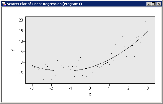
A Typical Scatter-diagram for a Quadratic Model

Enter your up-to-84 sample paired-data sets (X, Y), and then click the Calculate button. Blank boxes are not included in the calculations but zeros are.

Notice: The JavaScript enables you to perform serial-residual analysis provided you enter the independent variable X in increasing order.

In entering your data to move from cell to cell in the data-matrix use the Tab key not arrow or enter keys.

To edit your data, including add/change/delete, you do not have to click on the "clear" button, and re-enter your data all over again. You may simply add a number to any blank cell, change a number to another in the same cell, or delete a number from a cell. After editing, then click the "calculate" button.

For extensive edit or to use the JavaScript for a new set of data, then use the "clear" button.

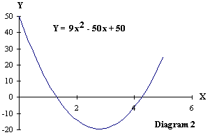
Calculus of Quadratic Functions: The following is a very basic review of introductory calculus concepts using a quadratic function example: Y = 9 X2 - 50 X + 50, which is graphed in following diagram. This function has a slope at every point. If we take the derivative of our quadratic function, we obtain a new function, Y' = 18 X - 50, which is graphed next to the diagram of the function, 2. The derivative function gives us the value of the slope (i.e., marginal value, rate of change) of our quadratic function at every point. Thus at X = 2, the slope of the quadratic function is 18(2)- 50 = -14.

A Quadratic Model
Click on the Image to View It
A Quadratic Model


Its Drivative Function
Click on the Image to View It
Its Drivative Function

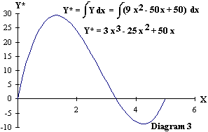
If on the other hand we integrate our quadratic function, we obtain a new function (Y* = 3 X3 - 25 X2 + 50 X), which is graphed below. The integrated function tells us the net area under the curve function (between the function curve and the X-axis). It actually tells us the area between some beginning X-value and ending X-value (when we do what is called a definite integral). For the integrated function above, the initial X value is zero and the ending X-value is whatever value we choose. That is for X = 2, the area under the quadratic function curve between zero and 2 is: A = 3 (2)3 -25 (2)2 + 50 (2) = 24. Thus every y value on the curve in Integral is equal to the sum of the area under the curve in function up to that point.

Its Inegral Function
Click on the Image to View It
Its Inegral Function


1
2
3
4
5
6
7
8
9
10
11
12
13
14
Variable X
Variable Y
 
15
16
17
18
19
20
21
22
23
24
25
26
27
28
Variable X
Variable Y
 
29
30
31
32
33
34
35
36
37
38
39
40
41
42
Variable X
Variable Y
 
43
44
45
46
47
48
49
50
51
52
53
54
55
56
Variable X
Variable Y
 
57
58
59
60
61
62
63
64
65
66
67
68
69
70
Variable X
Variable Y
 
71
72
73
74
75
76
77
78
79
80
81
82
83
84
Variable X
Variable Y
 
Mean(X) Mean(Y)
Coef. of X Sq. Coef. of X
Intercept Residuals' Stand. Error
Diagnostic Tools for Data Transformation Decisions
R-Square F-Statistic
Mean Variance
Mean:
The first half
Mean:
The second half
Variance:
The first-half
Variance:
The second half
First order serial-correlation Second order serial-correlation
Durbin-Watson statistic Mean absolute errors
Normality Condition:
ith Residual:

Quadratic Calculus
A quadratic is a curve of the parabola family.
They are written in the format ax2+bx+c= y

X2 + X + = Y


The area bounded by the curve above the X-axis is: sq. units
The gradient of the curve at any point is:
The value of the curve occurs at co-ordinates:


For Technical Details, Back to:
Business Statistics


Kindly email your comments to:
Professor Hossein Arsham


Regresión Cuadrática para el Ajuste de Modelos de Forma Parabólica
Nota para los usuarios de habla hispana:
Modelos de regresiones Cuadráticos son normalmente usadas en áreas económicas tales como en la función de utilidad predicciones análisis de costo beneficio, etc. Este JavaScript proporciona modelos de regresión de parábola.
Antes de utilizar este JavaScript es necesario construir un diagrama de dispersión para sus datos.
Si mediante una inspección visual al diagrama de dispersión no se puede rechazar la existencia de un comportamiento en “forma parabólica”, usted puede usar este JavaScript, de lo contrario, esta misma inspección lo puede ayudar a determinar el modelo de regresión polinomial apropiado para ajustar sus datos.
Introduzca hasta 84 pares de datos (X, Y), y luego presione el botón Calculate (Calcular.) Los espacios en blanco no son asumidos como ceros ni incluidos en los cálculos, pero los números cero si se incluyen.
Nota: Este JavaScript le facilita a usted realizar Análisis de Series Residuales, siempre y cuando usted introduzca variables independientes X en orden creciente.
Mientras entre sus datos en la matriz, muévase de celda a celda usando la tecla Tab, no use la flecha o la tecla de entrada.
Para editar sus datos (incluyendo agregar, cambiar o borrar), usted no tiene que presionar el botón Clear (Limpiar) para vaciar la matriz e introducir los datos de nuevo. Usted puede simplemente agregar, cambiar o borrar números en cualquier celda. Después de editar, presione el botón Calculate (Calcular).
Para una edición de datos mas extensiva, o para usar la matriz para incluir nuevos datos utilice el botón Clear (Limpiar).
Los resultados que usted obtendrá de esta matriz son:
Mean (X) = Media (X)
Mean (Y) = Media (Y)
Coef. of X Sq. = Coeficiente de X al cuadrado
Coef. of X = Coeficiente de X
Intercept = Intercepto Residuals’ Standard Error = Resoduos de Error Estándar
Diagnostic Tools for Data Transformation Decisions = Herramientas Diagnósticas para Decisiones sobre Transformaciones de Datos
R- square = R al cuadrado
F- statistic = Estadístico F
Mean = Media
Variance = Varianza
Mean the fisrst half = Media de la Primera Mitad
Mean the second half = Media de la Segunda Mitad
Variance the fisrst half = Varianza de la Primera Mitad
Variance the second half = Varianza de la Segunda Mitad
Second order serial- correlation = Correlación de Serie de Segundo Grado
First order serial- correlation = Correlación de Serie de Primer Grado
Durbin- Watson Statistic = Estadístico Durbin- Watson
Mean Absolute Error = Error Absoluto de la Media
Normality Condition = Condición de Normalidad
Ith Residual = Iésimo Residuo

Para Detalles Técnicos y Aplicaciones, Vuelta a:
Razonamiento Estadístico para la Toma de Decisiones Gerenciales


MENU

Decision Tools in Economics & Finance


Probabilistic Modeling

 
Statistics


The Copyright Statement: The fair use, according to the 1996 Fair Use Guidelines for Educational Multimedia, of materials presented on this Web site is permitted for non-commercial and classroom purposes only.
This site may be translated and/or mirrored intact (including these notices), on any server with public access. All files are available at http://home.ubalt.edu/ntsbarsh/Business-stat for mirroring.

Kindly e-mail me your comments, suggestions, and concerns. Thank you.

Professor Hossein Arsham   


Back to:

Dr Arsham's Home Page


EOF: © 1994-2015.