Excel For Statistical Data Analysis
This is a webtext companion site of
Business Statistics
USA Site
Para mis visitantes del mundo de habla hispana, este sitio se encuentra disponible en español en:
Sitio Espejo para América Latina
Sitio de los E.E.U.U.
Excel is the widely used statistical package, which serves as a tool to understand statistical concepts and computation to check your hand-worked calculation in solving your homework problems. The site provides an introduction to understand the basics of and working with the Excel. Redoing the illustrated numerical examples in this site will help improving your familiarity and as a result increase the effectiveness and efficiency of your process in statistics.
To search the site, try Edit | Find in page [Ctrl + f]. Enter a word or phrase in the dialogue box, e.g. "variance" or "mean" If the first appearance of the word/phrase is not what you are looking for, try Find Next.
MENU
- Introduction
- Entering Data
- Descriptive Statistics
- Normal Distribution
- Confidence Interval for the Mean
- Test of Hypothesis Concerning the Population Mean
- Difference Between Mean of Two Populations
- ANOVA: Analysis of Variances
- Goodness-of-Fit Test for Discrete Random Variables
- Test of Independence: Contingency Tables
- Test Hypothesis Concerning the Variance of Two Populations
- Linear Correlation and Regression Analysis
- Moving Average and Exponential Smoothing
- Applications and Numerical Examples
- Microsoft Excel Add-Ins for Solving Linear Programs
- Computer-assisted Learning: E-Labs and Computational Tools
- Interesting and Useful Sites
Companion Sites:
Introduction
This site provides illustrative experience in the use of Excel for data summary, presentation, and for other basic statistical analysis. I believe the popular use of Excel is on the areas where Excel really can excel. This includes organizing data, i.e. basic data management, tabulation and graphics. For real statistical analysis on must learn using the professional commercial statistical packages such as SAS, and SPSS.
Microsoft Excel 2000 (version 9) provides a set of data analysis tools called the Analysis ToolPak which you can use to save steps when you develop complex statistical analyses. You provide the data and parameters for each analysis; the tool uses the appropriate statistical macro functions and then displays the results in an output table. Some tools generate charts in addition to output tables.
If the Data Analysis command is selectable on the Tools menu, then the Analysis ToolPak is installed on your system. However, if the Data Analysis command is not on the Tools menu, you need to install the Analysis ToolPak by doing the following:
Step 1: On the Tools menu, click Add-Ins.... If Analysis ToolPak is not listed in the Add-Ins dialog box, click Browse and locate the drive, folder name, and file name for the Analysis ToolPak Add-in Analys32.xll usually located in the Program Files\Microsoft Office\Office\Library\Analysis folder. Once you find the file, select it and click OK.
Step 2: If you don't find the Analys32.xll file, then you must install it.
- Insert your Microsoft Office 2000 Disk 1 into the CD ROM drive.
- Select Run from the Windows Start menu.
- Browse and select the drive for your CD. Select Setup.exe, click Open, and click OK.
- Click the Add or Remove Features button.
- Click the + next to Microsoft Excel for Windows.
- Click the + next to Add-ins.
- Click the down arrow next to Analysis ToolPak.
- Select Run from My Computer.
- Select the Update Now button.
- Excel will now update your system to include Analysis ToolPak.
- Launch Excel.
- On the Tools menu, click Add-Ins... - and select the Analysis ToolPak check box.
Step 3: The Analysis ToolPak Add-In is now installed and Data Analysis... will now be selectable on the Tools menu.
Microsoft Excel is a powerful spreadsheet package available for Microsoft Windows and the Apple Macintosh. Spreadsheet software is used to store information in columns and rows which can then be organized and/or processed. Spreadsheets are designed to work well with numbers but often include text. Excel organizes your work into workbooks; each workbook can contain many worksheets; worksheets
are used to list and analyze data .
Excel is available on all public-access PCs (i.e., those, e.g., in the Library and PC Labs). It can be opened either by selecting Start - Programs - Microsoft Excel or by clicking on the Excel Short Cut which is either on your desktop, or on any PC, or on the Office Tool bar.
Opening a Document:
- Click on File-Open (Ctrl+O) to open/retrieve an existing workbook; change the directory area or drive to look for files in other locations
- To create a new workbook, click on File-New-Blank Document.
Saving and Closing a Document:
To save your document with its current filename, location and file format either click on File - Save. If you are saving for the first time, click File-Save; choose/type a name for your document; then click OK. Also use File-Save if you want to save to a different filename/location.
When you have finished working on a document you should close it. Go to the File menu and click on Close. If you have made any changes since the file was last saved, you will be asked if you wish to save them.
The Excel screen
Workbooks and worksheets:
When you start Excel, a blank worksheet is displayed which consists of a multiple grid of cells with numbered rows down the page and alphabetically-titled columns across the page. Each cell is referenced by its coordinates (e.g., A3 is used to refer to the cell in column A and row 3; B10:B20 is used to refer to the range
of cells in column B and rows 10 through 20).
Your work is stored in an Excel file called a workbook. Each workbook may contain several worksheets and/or charts - the current worksheet is called the active sheet. To view a different worksheet in a workbook click the appropriate Sheet Tab.
You can access and execute commands directly from the main menu or you can point to one of the toolbar buttons (the display box that appears below the button, when you place the cursor over it, indicates the name/action of the button) and click once.
Moving Around the Worksheet:
It is important to be able to move around the worksheet effectively because you can only enter or change data at the position of the cursor. You can move the cursor by using the arrow keys or by moving the mouse to the required cell and clicking. Once selected the cell becomes the active cell and is identified by a thick border; only one cell can be active at a time.
To move from one worksheet to another click the sheet tabs. (If your workbook contains many sheets, right-click the tab scrolling buttons then click the sheet you want.) The name of the active sheet is shown in bold.
Moving Between Cells:
Here is a keyboard shortcuts to move the active cell:
- Home - moves to the first column in the current row
- Ctrl+Home - moves to the top left corner of the document
- End then Home - moves to the last cell in the document
To move between cells on a worksheet, click any cell or use the arrow keys. To see a different area of the sheet, use the scroll bars and click on the arrows or the area above/below the scroll box in either the vertical or horizontal scroll bars.
Note that the size of a scroll box indicates the proportional amount of the used area of the sheet that is visible in the window. The position of a scroll box indicates the relative location of the visible area within the worksheet.
Entering Data
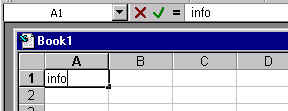
A new worksheet is a grid of rows and columns. The rows are labeled with numbers, and the columns are labeled with letters. Each intersection of a row and a column is a cell. Each cell has an address, which is the column letter and the row number. The arrow on the worksheet to the right points to cell A1, which is currently highlighted, indicating that it is an active cell. A cell must be active to enter information into it. To highlight (select) a cell, click on it.
To select more than one cell:
- Click on a cell (e.g. A1), then hold the shift key while you click on another (e.g. D4) to select all cells
between and including A1 and D4.
- Click on a cell (e.g. A1) and drag the mouse across the desired range, unclicking on another cell (e.g. D4) to select all cells between and including A1 and D4.
- To select several cells which are not adjacent, press "control" and click on the cells you want to select. Click a number or letter labeling a row or column to select that entire row or column.
One worksheet can have up to 256 columns and 65,536 rows, so it'll be a while before you run out of space.
Each cell can contain a label, value, logical value, or formula.
- Labels can contain any combination of letters, numbers, or
symbols.
- Values are numbers. Only values (numbers) can be used in calculations. A value can also be a date or a time
- Logical values are "true" or "false."
- Formulas automatically do calculations on the values in other specified cells and display the result in the cell in which the formula is entered (for example, you can specify that cell D3 is
to contain the sum of the numbers in B3 and C3; the number
displayed in D3 will then be a funtion of the numbers entered into
B3 and C3).
To enter information into a cell, select the cell and begin typing.
Note that as you type information into the cell, the information you enter also displays in the formula bar. You can also enter information into the formula bar, and the information will appear in the selected cell.
When you have finished entering the label or value:
- Press "Enter" to move to the next cell below (in this case, A2)
- Press "Tab" to move to the next cell to the right (in this case, B1)
- Click in any cell to select it
Entering Labels
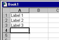
Unless the information you enter is formatted as a value or a formula, Excel will interpret it as a label, and
defaults to align the text on the left side of the cell.
If you are creating a long worksheet and you will be repeating the same label information in many different cells, you can use the AutoComplete function. This function will look at other entries in the same column and attempt to match a previous entry with your current entry. For example, if you have already typed "Wesleyan" in another cell and you type "W" in a new cell, Excel will automatically enter "Wesleyan." If you intended to type "Wesleyan" into the cell, your task is done, and you can move on to the next
cell. If you intended to type something else, e.g. "Williams," into the cell, just continue typing to enter the term.
To turn on the AutoComplete funtion, click on "Tools" in the menu bar, then select "Options," then select "Edit," and click to put a check in the box beside "Enable AutoComplete for cell values."
Another way to quickly enter repeated labels is to use the Pick List feature. Right click on a cell, then select "Pick From List." This will give you a menu of all other entries in cells in that column. Click on an item in the menu to enter it into the currently selected cell.
Entering Values
A value is a number, date, or time, plus a few symbols if necessary to further define the numbers [such as: . , + - ( ) % $ / ].
Numbers are assumed to be positive; to enter a negative number, use a minus sign "-" or enclose the number in parentheses "()".
Dates are stored as MM/DD/YYYY, but you do not have to enter it precisely in that format. If you enter "jan 9" or "jan-9", Excel will recognize it at January 9 of the current year, and store it as 1/9/2002. Enter the four-digit year for a year other than the current year (e.g. "jan 9, 1999"). To enter the current day's date,
press "control" and ";" at the same time.
Times default to a 24 hour clock. Use "a" or "p" to indicate "am" or "pm" if you use a 12 hour clock (e.g. "8:30 p" is interpreted as 8:30 PM). To enter the current time, press "control"
and ":" (shift-semicolon) at the same time.
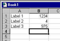
An entry interpreted as a value (number, date, or time) is aligned to the right side of the cell, to reformat a value.
Rounding Numbers that Meet Specified Criteria: To apply colors to maximum and/or minimum values:
- Select a cell in the region, and press Ctrl+Shift+* (in Excel 2003, press this or Ctrl+A) to select the Current Region.
- From the Format menu, select Conditional Formatting.
- In Condition 1, select Formula Is, and type =MAX($F:$F) =$F1.
- Click Format, select the Font tab, select a color, and then click OK.
- In Condition 2, select Formula Is, and type =MIN($F:$F) =$F1.
- Repeat step 4, select a different color than you selected for Condition 1, and then click OK.
Note: Be sure to distinguish between absolute reference and relative reference when entering the formulas.
Rounding Numbers that Meet Specified Criteria
Problem: Rounding all the numbers in column A to zero decimal places, except for those that have "5" in the first decimal place.
Solution: Use the IF, MOD, and ROUND functions in the following formula:
=IF(MOD(A2,1)=0.5,A2,ROUND(A2,0))
To Copy and Paste All Cells in a Sheet
- Select the cells in the sheet by pressing Ctrl+A (in Excel 2003, select a cell in a blank area before pressing Ctrl+A, or from a selected cell in a Current Region/List range, press Ctrl+A+A).
OR
Click Select All at the top-left intersection of rows and columns.
- Press Ctrl+C.
- Press Ctrl+Page Down to select another sheet, then select cell A1.
- Press Enter.
To Copy the Entire Sheet
Copying the entire sheet means copying the cells, the page setup parameters, and the defined range Names.
Option 1:
- Move the mouse pointer to a sheet tab.
- Press Ctrl, and hold the mouse to drag the sheet to a different location.
- Release the mouse button and the Ctrl key.
Option 2:
- Right-click the appropriate sheet tab.
- From the shortcut menu, select Move or Copy. The Move or Copy dialog box enables one to copy the sheet either to a different location in the current workbook or to a different workbook. Be sure to mark the Create a copy checkbox.
Option 3:
- From the Window menu, select Arrange.
- Select Tiled to tile all open workbooks in the window.
- Use Option 1 (dragging the sheet while pressing Ctrl) to copy or move a sheet.
Sorting by Columns
The default setting for sorting in Ascending or Descending order is by row. To sort by columns:
- From the Data menu, select Sort, and then Options.
- Select the Sort left to right option button and click OK.
- In the Sort by option of the Sort dialog box, select the row number by which the columns will be sorted and click OK.
Descriptive Statistics
The Data Analysis ToolPak has a Descriptive Statistics tool that provides you with an easy way to calculate summary statistics for a set of sample data. Summary statistics includes Mean, Standard Error, Median, Mode, Standard Deviation, Variance, Kurtosis, Skewness, Range, Minimum, Maximum, Sum, and Count. This tool eliminates the need to type indivividual functions to find each of these results. Excel includes elaborate and customisable toolbars, for example the "standard" toolbar shown here:

Some of the icons are useful mathematical computation:
 is the "Autosum" icon, which enters the formula "=sum()" to add up a range of cells.
 is the "FunctionWizard" icon, which
gives you access to all the functions available.
is the "FunctionWizard" icon, which
gives you access to all the functions available.
 is the "GraphWizard" icon, giving access to all graph types available, as shown in this display:
Excel can be used to generate measures of location and variability for a variable. Suppose we wish to find descriptive statistics for a sample data: 2, 4, 6, and 8.
Step 1. Select the Tools *pull-down menu, if you see data analysis, click on this option, otherwise, click on add-in.. option to install analysis tool pak.
Step 2. Click on the data analysis option.
Step 3. Choose Descriptive Statistics from Analysis Tools list.
Step 4. When the dialog box appears:
Enter A1:A4 in the input range box, A1 is a value in column A and row 1, in this case this value is 2. Using the same technique enter other VALUES until you reach the last one. If a sample consists of 20 numbers, you can select for example A1, A2, A3, etc. as the input range.
Step 5. Select an output range, in this case B1. Click on summary statistics to see the results.
Select OK.
When you click OK, you will see the result in the selected range.
As you will see, the mean of the sample is 5, the median is 5, the standard deviation is 2.581989, the sample variance is 6.666667,the range is 6 and so on. Each of these factors might be important in your calculation
of different statistical procedures.
Normal Distribution
Consider the problem of finding the probability of getting less than a certain value under any normal probability distribution. As an illustrative example, let us suppose the SAT scores nationwide are normally distributed with a mean and standard deviation of 500 and 100, respectively. Answer the following questions based on the given information:
A: What is the probability that a randomly selected student score will be less than 600 points?
B: What is the probability that a randomly selected student score will exceed 600 points?
C: What is the probability that a randomly selected student score will be between 400 and 600?
Hint: Using Excel you can find the probability of getting a value approximately less than or equal to a given value. In a problem, when the mean and the standard deviation of the population are given, you have to use common sense to find different probabilities based on the question since you know the area under a normal curve is 1.
Solution:
In the work sheet, select the cell where you want the answer to appear. Suppose, you chose cell number one, A1. From the menus, select "insert pull-down".
Steps 2-3 From the menus, select insert, then click on the Function option.
Step 4. After clicking on the Function option, the Paste Function dialog appears from Function Category. Choose Statistical then NORMDIST from the Function Name box; Click OK
Step 5. After clicking on OK, the NORMDIST distribution box appears:
i. Enter 600 in X (the value box);
ii. Enter 500 in the Mean box;
iii. Enter 100 in the Standard deviation box;
iv. Type "true" in the cumulative box, then click OK.
As you see the value 0.84134474 appears in A1, indicating the probability that a randomly selected student's score is below 600 points. Using common sense we can answer part "b" by subtracting 0.84134474 from 1. So the part "b" answer is 1- 0.8413474 or 0.158653. This is the probability that a randomly selected student's score is greater than 600 points. To answer part "c", use the same techniques to find the probabilities or area in the left sides of values 600 and 400. Since these areas or probabilities overlap each other to answer the question you should subtract the smaller probability from the larger probability. The answer equals 0.84134474 - 0.15865526 that is, 0.68269. The screen shot should look like following:
Inverse Case
Calculating the value of a random variable often called the "x" value
You can use NORMINV from the function box to calculate a value for the random variable - if the probability to the left side of this variable is given. Actually, you should use this function to calculate different percentiles. In this problem one could ask what is the score of a student whose percentile is 90? This means approximately 90% of students scores are less than this number. On the other hand if we were asked to do this problem by hand, we would have had to calculate the x value using the normal distribution formula x = m + zd. Now let's use Excel to calculate P90. In the Paste function, dialog click on statistical, then click on NORMINV. The screen shot would look like the following:
When you see NORMINV the dialog box appears.
i. Enter 0.90 for the probability (this means that approximately 90% of students' score is less than the value we are looking for)
ii. Enter 500 for the mean (this is the mean of the normal distribution in our case)
iii. Enter 100 for the standard deviation (this is the standard deviation of the normal distribution in our case)
At the end of this screen you will see the formula result which is approximately 628 points. This means the top 10% of the students scored better than 628.
Confidence Interval for the Mean
Suppose we wish for estimating a confidence interval for the mean of a population. Depending on the size of your sample size you may use one of the following cases:
Large Sample Size (n is larger than, say 30):
The general formula for developing a confidence interval for a population means is:
In this formula  is the mean of the sample; Z is the interval coefficient, which can be found from the normal distribution table (for example the interval coefficient for a 95% confidence level is 1.96). S is the standard deviation of the sample and n is the sample size.
Now we would like to show how Excel is used to develop a certain confidence interval of a population mean based on a sample information. As you see in order to evaluate this formula you need "the mean of the sample" and the margin of error  Excel will automatically calculate these quantities for you.
The only things you have to do are:
add the margin of error to the mean of the sample, ; Find the upper limit of the interval and subtract the margin of error from the mean to the lower limit of the interval. To demonstrate how Excel finds these quantities we will use the data set, which contains the hourly income of 36 work-study students here, at the University of Baltimore. These numbers appear in cells A1 to A36 on an Excel work sheet.
After entering the data, we followed the descriptive statistic procedure to calculate the unknown quantities. The only additional step is to click on the confidence interval in the descriptive statistics dialog box and enter the given confidence level, in this case 95%.
Here is, the above procedures in step-by-step:
Step 1. Enter data in cells A1 to A36 (on the spreadsheet)
Step 2. From the menus select Tools
Step 3. Click on Data Analysis then choose the Descriptive Statistics option then click OK.
On the descriptive statistics dialog, click on Summary Statistic. After you have done that, click on the confidence interval level and type 95% - or in other problems whatever confidence interval you desire. In the Output Range box enter B1 or what ever location you desire.
Now click on OK. The screen shot would look like the following:
As you see, the spreadsheet shows that the mean of the sample is = 6.902777778 and the absolute value of the margin of error  = 0.231678109. This mean is based on this sample information. A 95% confidence interval for the hourly income of the UB work-study students has an upper limit of 6.902777778 + 0.231678109 and a lower limit of 6.902777778 - 0.231678109.
On the other hand, we can say that of all the intervals formed this way 95% contains the mean of the population. Or, for practical purposes, we can be 95% confident that the mean of the population is between 6.902777778 - 0.231678109 and 6.902777778 + 0.231678109. We can be at least 95% confident that interval [$6.68 and $7.13] contains the average hourly income of a work-study student.
Smal Sample Size (say less than 30)
If the sample n is less than 30 or we must use the small sample procedure to develop a confidence interval for the mean of a population. The general formula for developing confidence intervals for the population mean based on small a sample is:
In this formula is the mean of the sample.  is the interval coefficient providing an area of
  in the upper tail of a t distribution with n-1 degrees of freedom which can be found from a t distribution table (for example the interval coefficient for a 90% confidence level is 1.833 if the sample is 10). S is the standard deviation of the sample and n is the sample size.
Now you would like to see how Excel is used to develop a certain confidence interval of a population mean based on this small sample information.
As you see, to evaluate this formula you need "the mean of the sample" and the margin of error  Excel will automatically calculate these quantities the way it did for large samples.
Again, the only things you have to do are: add the margin of error to the mean of the sample,, find the upper limit of the interval and to subtract the margin of error from the mean to find the lower limit of the interval.
To demonstrate how Excel finds these quantities we will use the data set, which contains the hourly incomes of 10 work-study students here, at the University of Baltimore. These numbers appear in cells A1 to A10 on an Excel work sheet.
After entering the data we follow the descriptive statistic procedure to calculate the unknown quantities (exactly the way we found quantities for large sample). Here you are with the procedures in step-by-step form:
Step 1. Enter data in cells A1 to A10 on the spreadsheet
Step 2. From the menus select Tools
Step 3. Click on Data Analysis then choose the Descriptive Statistics option. Click OK on the descriptive statistics dialog, click on Summary Statistic, click on the confidence interval level and type in 90% or in other problems whichever confidence interval you desire. In the Output Range box, enter B1 or whatever location you desire. Now click on OK. The screen shot will look like the following:
Now, like the calculation of the confidence interval for the large sample, calculate the confidence interval of the population based on this small sample information. The confidence interval is:
6.8 ± 0.414426102
or
$6.39<===>$7.21.
We can be at least 90% confidant that the interval [$6.39 and $7.21] contains the true mean of the population.
Test of Hypothesis Concerning the Population Mean
Again, we must distinguish two cases with respect to the size of your sample
Large Sample Size (say, over 30):
In this section you wish to know how Excel can be used to conduct a hypothesis test about a population mean. We will use the hourly incomes of different work-study students than those introduced earlier in the confidence interval section. Data are entered in cells A1 to A36. The objective is to test the following Null and Alternative hypothesis:

The null hypothesis indicates that the average hourly income of a work-study student is equal to $7 per hour; however, the alternative hypothesis indicates that the average hourly income is not equal to $7 per hour.
I will repeat the steps taken in descriptive statistics and at the very end will show how to find the value of the test statistics in this case, z, using a cell formula.
Step 1. Enter data in cells A1 to A36 (on the spreadsheet)
Step 2. From the menus select Tools
Step 3. Click on Data Analysis then choose the Descriptive Statistics option, click OK.
On the descriptive statistics dialog, click on Summary Statistic. Select the Output Range box, enter B1 or whichever location you desire. Now click OK.
(To calculate the value of the test statistics search for the mean of the sample then the standard error. In this output, these values are in cells C3 and C4.)
Step 4. Select cell D1 and enter the cell formula = (C3 - 7)/C4. The screen shot should look like the following:
The value in cell D1 is the value of the test statistics. Since this value falls in acceptance range of -1.96 to 1.96 (from the normal distribution table), we fail to reject the null hypothesis.
Small Sample Size (say, less than 30):
Using steps taken the large sample size case, Excel can be used to conduct a hypothesis for small-sample case. Let's use the hourly income of 10 work-study students at UB to conduct the following hypothesis.
The null hypothesis indicates that average hourly income of a work-study student is equal to $7 per hour .The alternative hypothesis indicates that average hourly income is not equal to $7 per hour.
I will repeat the steps taken in descriptive statistics and at the very end will show how to find the value of the test statistics in this case "t" using a cell formula.
Step 1. Enter data in cells A1 to A10 (on the spreadsheet)
Step 2. From the menus select Tools
Step 3. Click on Data Analysis then choose the Descriptive Statistics option. Click OK.
On the descriptive statistics dialog, click on Summary Statistic. Select the Output Range boxes, enter B1 or whatever location you chose. Again, click on OK.
(To calculate the value of the test statistics search for the mean of the sample then the standard
error, in this output these values are in cells C3 and C4.)
Step 4. Select cell D1 and enter the cell formula = (C3 - 7)/C4. The screen shot would look like the following:
Since the value of test statistic t = -0.66896 falls in acceptance range -2.262 to +2.262 (from t table, where = 0.025 and the degrees of freedom is 9), we fail to reject the null hypothesis.
Difference Between Mean of Two Populations
In this section we will show how Excel is used to conduct a hypothesis test about the difference between two population means assuming that populations have equal variances. The data in this case are taken from various offices here at the University of Baltimore. I collected the hourly income data of 36 randomly selected work-study students and 36 student assistants. The hourly income range for work-study students was $6 - $8 while the hourly income range for student assistants was $6-$9. The main objective in this hypothesis testing is to see whether there is a significant difference between the means of the two populations. The NULL and the ALTERNATIVE hypothesis is that the means are equal and the means are not equal, respectively.
Referring to the spreadsheet, I chose A1 and A2 as label centers. The work-study students' hourly income for a sample size 36 are shown in cells A2:A37, and the student assistants' hourly income for a sample size 36 is shown in cells B2:B37
Data for Work Study Student: 6, 6, 6, 6, 6, 6, 6, 6.5, 6.5, 6.5, 6.5, 6.5, 6.5, 7, 7, 7, 7, 7, 7, 7, 7.5, 7.5, 7.5, 7.5, 7.5, 7.5, 8, 8, 8, 8, 8, 8, 8, 8, 8.
Data for Student Assistant: 6, 6, 6, 6, 6, 6.5, 6.5, 6.5, 6.5, 6.5, 7, 7, 7, 7, 7, 7.5, 7.5, 7.5, 7.5, 7.5, 7.5, 8, 8, 8, 8, 8, 8, 8, 8.5, 8.5, 8.5, 8.5, 8.5, 9, 9, 9, 9.
Use the Descriptive Statistics procedure to calculate the variances of the two samples. The Excel procedure for testing the difference between the two population means will require information on the variances of the two populations. Since the variances of the two populations are unknowns they should be replaced with sample variances. The descriptive for both samples show that the variance of first sample is s12 = 0.55546218, while the variance of the second sample s22 =0.969748.
| work-study student |
|
student assistant |
|
|
|
|
|
| Mean |
7.05714286 |
Mean |
7.471429 |
| Standard Error |
0.12597757 |
Standard Error |
0.166454 |
| Median |
7 |
Median |
7.5 |
| Mode |
8 |
Mode |
8 |
| Standard Deviation |
0.74529335 |
Standard Deviation |
0.984758 |
| Sample Variance |
0.55546218 |
Sample Variance |
0.969748 |
| Kurtosis |
-1.38870558 |
Kurtosis |
-1.192825 |
| Skewness |
-0.09374375 |
Skewness |
-0.013819 |
| Range |
2 |
Range |
3 |
| Minimum |
6 |
Minimum |
6 |
| Maximum |
8 |
Maximum |
9 |
| Sum |
247 |
Sum |
261.5 |
| Count |
35 |
Count |
35 |
To conduct the desired test hypothesis with Excel the following steps can be taken:
Step 1. From the menus select Tools then click on the Data Analysis option.
Step 2. When the Data Analysis dialog box appears:
Choose z-Test: Two Sample for means then click OK
Step 3. When the z-Test: Two Sample for means dialog box appears:
Enter A1:A36 in the variable 1 range box (work-study students' hourly income)
Enter B1:B36 in the variable 2 range box (student assistants' hourly income)
Enter 0 in the Hypothesis Mean Difference box (if you desire to test a mean difference other than 0, enter that value)
Enter the variance of the first sample in the Variable 1 Variance box
Enter the variance of the second sample in the Variable 2 Variance box and select Labels
Enter 0.05 or, whatever level of significance you desire, in the Alpha box
Select a suitable Output Range for the results, I chose C19, then click OK.
The value of test statistic z=-1.9845824 appears in our case in cell D24. The rejection rule for this test is z < -1.96 or z > 1.96 from the normal distribution table. In the Excel output these values for a two-tail test
are z<-1.959961082 and z>+1.959961082. Since the value of the test statistic z=-1.9845824 is less than -1.959961082 we reject the null hypothesis. We can also draw this conclusion by comparing the p-value for a two tail -test and the alpha value.
Since p-value 0.047190813 is less than a=0.05 we reject the null hypothesis. Overall we can say, based on the sample results, the two populations' means are different.
Small Samples: n1 OR n2 are less than 30
In this section we will show how Excel is used to conduct a hypothesis test about the difference between two population means. - Given that the populations have equal variances when two small independent samples are taken from both populations. Similar to the above case, the data in this case are taken from various offices here at the University of Baltimore. I collected hourly income data of 11 randomly selected work-study students and 11 randomly selected student assistants. The hourly income range for both groups was similar range, $6 - $8 and $6-$9. The main objective in this hypothesis testing is similar too, to see whether there is a significant difference between the means of the two populations. The NULL and the ALTERNATIVE hypothesis are that the means are equal and they are not equal, respectively.
| work-study student |
student assistant |
| 6 |
6 |
| 8 |
9 |
| 7.5 |
8.5 |
| 6.5 |
7 |
| 7 |
6.5 |
| 6 |
7 |
| 7.5 |
7.5 |
| 8 |
6 |
| 6 |
8 |
| 6.5 |
9 |
| 7 |
7.5> |
Referring to the spreadsheet, we chose A1 and A2 as label centers. The work-study students' hourly income for a sample size 11 are shown in cells A2:A12, and the student assistants' hourly income for a sample size 11 is shown in cells B2:B12. Unlike previous case, you do not have to calculate the variances of the two samples, Excel will automatically calculate these quantities and use them in the calculation of the value of the test statistic.
Similar to the previous case, but a bit different in step # 2, to conduct the desired test hypothesis with Excel the following steps can be taken:
Step 1. From the menus select Tools then click on the Data Analysis option.
Step 2. When the Data Analysis dialog box appears:
Choose t-Test: Two Sample Assuming Equal Variances then click OK
Step 3 When the t-Test: Two Sample Assuming Equal Variances dialog box appears:
Enter A1:A12 in the variable 1 range box (work-study student hourly income)
Enter B1:B12 in the variable 2 range box (student assistant hourly income)
Enter 0 in the Hypothesis Mean Difference box(if you desire to test a mean difference other than zero, enter that value) then select Labels
Enter 0.05 or, whatever level of significance you desire, in the Alpha box
Select a suitable Output Range for the results, I chose C1, then click OK.
The value of the test statistic t=-1.362229828 appears, in our case, in cell D10. The rejection rule for this test is t<-2.086 or t>+2.086 from the t distribution table where the t value is based on a t distribution with n1-n2-2 degrees of freedom and where the area of the upper one tail is 0.025 ( that is equal to alpha/2).
In the Excel output the values for a two-tail test are t<-2.085962478 and t>+2.085962478. Since the value of the test statistic t=-1.362229828, is in an acceptance range of t<-2.085962478 and t>+2.085962478, we fail to reject the null hypothesis.
We can also draw this conclusion by comparing the p-value for a two-tail test and the alpha value.
Since the p-value 0.188271278 is greater than a=0.05 again, we fail to reject the null hypothesis.
Overall we can say, based on sample results, the two populations' means are equal.
|
work-study student |
student assistant |
| Mean |
6.909090909 |
7.454545455 |
| Variance |
0.590909091 |
1.172727273 |
| Observations |
11 |
11 |
| Pooled Variance |
0.881818182 |
|
| Hypothesized Mean Difference |
0 |
|
| Df |
20 |
|
| t Stat |
-1.362229828 |
|
| P(T<=t) one tail |
0.094135639 |
|
| t Critical one tail |
1.724718004 |
|
| P(T<=t)two tail |
0.188271278 |
|
| t Critical two tail |
2.085962478 |
|
ANOVA: Analysis of Variances
In this section the objective is to see whether or not means of three or more populations based on random samples taken from populations are equal or not. Assuming independents samples are taken from normally distributed populations with equal variances, Excel would do this analysis if you choose one way anova from the menus. We can also choose Anova: two way factor with or without replication option and see whether there is significant difference between means when different factors are involved.
Single-Factor ANOVA Test
In this case we were interested to see whether there a significant difference among hourly wages of student assistants in three different service departments here at the University of Baltimore. Six student assistants were randomly were selected from the three departments and their hourly wages were recorded as following:
| ARC | CSI | TCC |
| 10.00 | 6.50 | 9.00 |
| 8.00 | 7.00 | 7.00 |
| 7.50 | 7.00 | 7.00 |
| 8.00 | 7.50 | 7.00 |
| 7.00 | 7.00 | 6.50 |
Enter data in an Excel work sheet starting with cell A2 and ending with cell C8. The following steps should be taken to find the proper output for interpretation.
Step 1. From the menus select Tools and click on Data Analysis option.
Step 2. When data analysis dialog appears, choose Anova single-factor option; enter A2:C8 in the input range box. Select labels in first row.
Step3.Select any cell as output(in here we selected A11). Click OK.
The general form of Anova table looks like following:
| Source of Variation |
SS |
df |
MS |
F |
P-value |
F crit |
| Between Groups |
SSTR |
K-1 |
MSTR |
MST/MSE |
0.046725 |
3.682316674 |
| Within Groups |
SSE |
nt-K |
MSE |
|
|
|
| Total |
Suppose the test is done at level of significance a = 0.05, we reject the null hypothesis. This means there is a significant difference between means of hourly incomes of student assistants in these departments.
The Two-way ANOVA Without Replication
In this section, the study involves six students who were offered different hourly wages in three different department services here at the University of Baltimore. The objective is to see whether the hourly incomes are the same. Therefore, we can consider the following:
Factor: Department
Treatment: Hourly payments in the three departments
Blocks: Each student is a block since each student has worked in the three different departments
| Student |
ARC |
CSI |
TCC |
|
|
|
|
| 1 |
10.00 |
7.50 |
7.00 |
| 2 |
8.00 |
7.00 |
6.00 |
| 3 |
7.00 |
6.00 |
6.00 |
| 4 |
8.00 |
6.50 |
6.50 |
| 5 |
9.00 |
8.00 |
7.00 |
| 6 |
8.00 |
8.00 |
6.00 |
The general form of Anova table would look like:
| Source of Variation |
Sum of Squares |
Degrees of freedom |
Mean Squares |
F |
|
|
|
|
|
| Treatment |
SST |
K-1 |
MST |
F=MST/MSE |
| Blocks |
SSB |
b-1 |
MSB |
|
| Error |
SSE |
(K-1)(b-1) |
MSB |
|
| Total |
SST |
nt-1 |
|
|
To find the Excel output for the above data the following steps can be taken:
Step 1. From the menus select Tools and click on Data Analysis option.
Step2. When data analysis box appears: select Anova two-factor without replication then Enter A2: D8 in the input range. Select labels in first row.
Step3. Select an output range (in here we selected A11) then OK.
| SUMMARY |
COUNT |
SUM |
AVERAGE |
VARIANCE |
| 1 |
3 |
24.5 |
8.166667 |
2.583333 |
| 2 |
3 |
21 |
7 |
1 |
| 3 |
3 |
19.5 |
6.5 |
0.25 |
| 4 |
3 |
21.5 |
7.166667 |
0.583333 |
| 5 |
3 |
23 |
7.666667 |
2.333333 |
| 6 |
3 |
22 |
7.333333 |
1.333333 |
|
|
|
|
|
| ARC |
6 |
50 |
8.333333 |
1.066667 |
| CSI |
6 |
43 |
7.166667 |
0.666667 |
| TCC |
6 |
38.5 |
6.416667 |
0.241667 |
ANOVA
| Source of Variation |
SS |
df |
MS |
F |
P-value |
F crit |
| Rows |
4.902778 |
5 |
0.980556 |
1.972067 |
0.168792 |
3.325837 |
| Columns |
11.19444 |
2 |
5.597222 |
11.25698 |
0.002752 |
4.102816 |
| Error |
4.972222 |
10 |
0.497222 |
|
|
|
|
|
|
|
|
|
|
| Total |
21.06944 |
17 |
|
|
|
|
NOTE: F=MST/MSE =0.980556/0.497222 = 1.972067
F = 3.33 from table (5 numerator DF and 10 denominator DF)
Since 1.972067<3.33 we fail to reject the null.
Conclusion: There is not sufficient evidence to conclude that hourly rates differ for the three departments.
Two-Way ANOVA with Replication
Referring to the student assistant and the work study hourly wages here at the university of Baltimore the following data shows the hourly wages for the two categories in three different departments:
| |
ARC |
CSI |
TCC |
| |
6.50 |
6.10 |
6.90 |
| Work Study |
6.80 |
6.00 |
7.20 |
| |
7.10 |
6.50 |
7.10 |
| |
7.40 |
6.80 |
7.50 |
| Student Assistant |
7.50 |
7.00 |
7.00 |
| |
8.00 |
6.60 |
7.10 |
|
|
|
|
| Factors |
|
|
|
Factor A: Student job category (in here two different job categories exists)
Factor B: Departments (in here we have three departments)
Replication: The number of students in each experimental condition. In this
case there are three replications.
Interaction:
|
ARC |
CSI |
TCC |
|
6.50 |
6.10 |
6.90 |
| Work Study |
6.80 |
6.00 |
7.20 |
|
7.10 |
6.50 |
7.10 |
|
7.40 |
6.80 |
7.50 |
| Student Assistant |
7.50 |
7.00 |
7.00 |
|
8.00 |
6.60 |
7.10 |
|
|
|
|
| SUMMARY |
ARC |
CSI |
TCC |
Total |
|
|
|
|
|
| Count |
3 |
3 |
3 |
9 |
| Sum |
20.4 |
19 |
21 |
60.2 |
| Average |
6.8 |
6.2 |
7.1 |
6.69 |
| Variance |
0.09 |
0.1 |
0 |
0.19 |
| Count |
3 |
3 |
3 |
9 |
| Sum |
22.9 |
20 |
22 |
64.9 |
| Average |
7.63333 |
6.8 |
7.2 |
7.21 |
| Variance |
0.10333 |
0 |
0.1 |
0.18 |
| Total |
|
|
|
|
|
Total |
|
|
| Count |
6 |
6 |
6 |
| Sum |
43.3 |
39 |
43 |
| Average |
7.21667 |
6.5 |
7.1 |
| Variance |
0.28567 |
0.2 |
0 |
ANOVA
| Source of Variation |
SS |
df |
MS |
F |
P-value |
F crit |
| Sample(Factor A) |
1.22722 |
1 |
1.2 |
18.6 |
0.001016557 |
4.747221 |
| Columns(Factor B) |
1.84333 |
2 |
0.9 |
13.9 |
0.000741998 |
3.88529 |
| Interaction |
0.38111 |
2 |
0.2 |
2.88 |
0.095003443 |
3.88529 |
| Within |
0.79333 |
12 |
0.1 |
|
|
|
|
|
|
|
|
|
|
| Total |
4.245 |
17 |
|
|
|
|
Conclusion:
Mean hourly income differ by job category.
Mean hourly income differ by department.
Interaction is not significant.
Goodness-of-Fit Test for Discrete Random Variables
The CHI-SQUARE distribution can be used in a hypothesis test involving a population variance. However, in this section we would like to test and see how close a sample results are to the expected results.
Example: The Multinomial Random Variable
In this example the objective is to see whether or not based on a randomly selected sample information the standards set for a population is met. There are so many practical examples that can be used in this situation. For example it is assumed the guidelines for hiring people with different ethnic background for the US government is set at 70%(WHITE), 20%(African American) and 10%(others), respectively. A randomly selected sample of 1000 US employees shows the following results that is summarized in a table.
| ETHNIC BACKGROUND |
EXPECTED NUMBER OF EMPLOYEES |
OBSERVED FROM SAMPLE |
| WHITE |
700 =70%OF 1000 |
750 |
| AFRICAN American |
200 =20%OF 1000 |
170 |
| OTHERS |
100 =10%OF 1000 |
80 |
As you see the observed sample numbers for groups two and three are lower than their expected values unlike group one which has a higher expected value. Is this a clear sign of discrimination with respect to ethnic background? Well depends on how much lower the expected values are. The lower amount might not statistically be significant. To see whether these differences are significant we can use Excel and find the value of the CHI-SQUARE. If this value falls within the acceptance region we can assume that the guidelines are met otherwise they are not. Now lets enter these numbers into Excel spread- sheet. We used cells B7-B9 for the expected proportions, C7-C9 for the observed values and D7-D9 for the expected frequency. To calculate the expected frequency for a category, you can multiply the proportion of that category by the sample size (in here 1000). The formula for the first cell of the expected value column, D7 is 1000*B7. To find other entries in the expected value column, use the copy and the paste menu as shown in the following picture. These are important values for the chi-square test. The observed range in this case is C7: C9 while the expected range is D7: D9. The null and the alternative hypothesis for this test are as follows:
H0 : PW = 0.70, PA=0.20 and PO =0.10
HA: The population proportions are not PW = 0.70, PA= 0.20 and PO = 0.10
Now lets use Excel to calculate the p-value in a CHI-SQUARE test.
Step 1.Select a cell in the work sheet, the location which you like the p value of the CHI-SQUARE to appear. We chose cell D12.
Step 2. From the menus, select insert then click on the Function option, Paste Function dialog box appears.
Step 3.Refer to function category box and choose statistical, from function name box select CHITEST and click on OK.
Step 4.When the CHITEST dialog appears:
Enter C7: C9 in the actual-range box then enter D7: D9 in the expected-range box, and finally click on OK.
The p-value will appear in the selected cell, D12.
As you see the p value is 0.002392 which is less than the value of the level of significance (in this case the level of significance, a= 0.10). Hence the null hypothesis should be rejected. This means based on the sample information the guidelines are not met.
Notice if you type "=CHITEST(C7:C9,D7:D9)" in the formula bar the p-value will show up in the designated cell.
NOTE: Excel can actually find the value of the CHI-SQUARE. To find this value first select an empty cell on the spread sheet then in the formula bar type "=CHIINV(D12,2)." D12 designates the p-Value found previously and 2 is the degrees of freedom (number of rows minus one). The CHI-SQUARE value in this case is 12.07121. If we refer to the CHI-SQUARE table we will see that the cut off is 4.60517 since 12.07121>4.60517 we reject the null. The following screen shot shows you how to the CHI-SQUARE value.
Test of Independence: Contingency Tables
The CHI-SQUARE distribution is also used to test and see whether two variables are independent or not. For example based on sample data you might want to see whether smoking and gender are independent events for a certain population. The variables of interest in this case are smoking and the gender of an individual. Another example in this situation could involve the age range of an individual and his or her smoking habit. Similar to case one data may appear in a table but unlike the case one this table may contains several columns in addition to rows. The initial table contains the observed values. To find expected values for this table we set up another table similar to this one. To find the value of each cell in the new table we should multiply the sum of the cell column by the sum of the cell row and divide the results by the grand total. The grand total is the total number of observations in a study. Now based on the following table test whether or not the smoking habit and gender of the population that the following sample taken from are independent. On the other hand is that true that males in this population smoke more than females?
You could use formula bar to calculate the expected values for the expected range. For example to find the expected value for the cell C5 which is replaced in c11 you could click on the formula bar and enter C6*D5/D6 then enter in cell C11.
Step 1. Observed Range b4:c5
Smoking and gender
|
yes |
no |
total |
| male |
31 |
69 |
100 |
| female |
45 |
122 |
167 |
| total |
76 |
191 |
267 |
Step2. Expected Range b10:c11
| 28.46442 |
71.53558 |
| 47.53558 |
119.4644 |
So the observed range is b4:c5 and the expected range is b10:c11.
Step 3. Click on fx(paste function)
Step 4. When Paste Function dialog box appears, click on Statistical in function category and CHITEST in the function name then click OK.
When the CHITEST box appears, enter b4:c5 for the actual range, then b10:c11 for the expected range.
Step 5. Click on OK (the p-value appears). 0.477395
Conclusion: Since p-value is greater than the level of significance (0.05), fails to reject the null. This means smoking and gender are independent events. Based on sample information one can not assure females smoke more than males or the other way around.
Step 6. To find the chi-square value, use CHINV function, when Chinv box appears enter 0.477395 for probability part, then 1 for the degrees of freedom.
Degrees of freedom=(number of columns-1)X(number of rows-1)
CHI-SQUARE=0.504807
Test Hypothesis Concerning the Variance of Two Populations
In this section we would like to examine whether or not the variances of two populations are equal. Whenever independent simple random samples of equal or different sizes such as n1 and n2 are taken from two normal distributions with equal variances, the sampling distribution of s12/s22 has F distribution with n1- 1 degrees of freedom for the numerator and n2 - 1 degrees of freedom for the denominator. In the ratio s12/s22 the numerator s12 and the denominator s22 are variances of the first and the second sample, respectively. The following figure shows the graph of an F distribution with 10 degrees of freedom for both the numerator and the denominator. Unlike the normal distribution as you see the F distribution is not symmetric. The shape of an F distribution is positively skewed and depends on the degrees of freedom for the numerator and the denominator. The value of F is always positive.
Now let see whether or not the variances of hourly income of student-assistant and work-study students based on samples taken from populations previously are equal. Assume that the hypothesis test in this case is conducted at a = 0.10. The null and the alternative are:
Rejection Rule: Reject the null hypothesis if F< F0.095 or F> F0.05 where F, the value of the test statistic is equal to s12/s22, with 10 degrees of freedom for both the numerator and the denominator. We can find the value of F.05 from the F distribution table. If s12/s22, we do not need to know the value of F0.095 otherwise, F0.95 = 1/ F0.05 for equal sample sizes.

A survey of eleven student-assistant and eleven work-study students shows the following
descriptive statistics. Our objective is to find the value of s12/s22, where s12 is the value of the variance of student assistant sample and s22 is the value of the variance of the work study students sample. As you see these values are in cells F8 and D8 of the descriptive statistic output.
To calculate the value of s12/s22, select a cell such as A16 and enter cell formula = F8/D8 and enter. This is the value of F in our problem. Since this value, F=1.984615385, falls in acceptance area we fail to reject the null hypothesis. Hence, the sample results do support the conclusion that student assistants hourly income variance is equal to the work study students hourly income variance. The following screen shoot shows how to find the F value. We can follow the same format for one tail test(s).
Linear Correlation and Regression Analysis
In this section the objective is to see whether there is a correlation between two variables and to find a model that predicts one variable in terms of the other variable. There are so many examples that we could mention but we will mention the popular ones in the world of business. Usually independent variable is presented by the letter x and the dependent variable is presented by the letter y. A business man would like to see whether there is a relationship between the number of cases of sold and the temperature in a hot summer day based on information taken from the past. He also would like to estimate the number cases of soda which will be sold in a particular hot summer day in a ball game. He clearly recorded temperatures and number of cases of soda sold on those particular days. The following table shows the recorded data from June 1 through June 13. The weatherman predicts a 94F degree temperature for June 14. The businessman would like to meet all demands for the cases of sodas ordered by customers on June 14.
| DAY |
Cases of Soda |
Temperature |
| 1-Jun |
57 |
56 |
| 2-Jun |
59 |
58 |
| 3-Jun |
65 |
63 |
| 4-Jun |
67 |
66 |
| 5-Jun |
75 |
73 |
| 6-Jun |
81 |
78 |
| 7-Jun |
86 |
85 |
| 8-Jun |
88 |
85 |
| 9-Jun |
88 |
87 |
| 10-Jun |
84 |
84 |
| 11-Jun |
82 |
88 |
| 12-Jun |
80 |
84 |
| 13-Jun |
83 |
89 |
Now lets use Excel to find the linear correlation coefficient and the regression line equation. The linear correlation coefficient is a quantity between -1 and +1. This quantity is denoted by R. The closer R to +1 the stronger positive (direct) correlation and similarly the closer R to -1 the stronger negative (inverse) correlation exists between the two variables. The general form of the regression line is y = mx + b. In this formula, m is the slope of the line and b is the y-intercept. You can find these quantities from the Excel output. In this situation the variable y (the dependent variable) is the number of cases of soda and the x (independent variable) is the temperature. To find the Excel output the following steps can be taken:
Step 1. From the menus choose Tools and click on Data Analysis.
Step 2. When Data Analysis dialog box appears, click on correlation.
Step 3. When correlation dialog box appears, enter B1:C14 in the input range box. Click on Labels in first row and enter a16 in the output range box. Click on OK.
|
Cases of Soda |
Temperature |
| Cases of Soda |
1 |
|
| Temperature |
0.96659877 |
1 |
As you see the correlation between the number of cases of soda demanded and the temperature is a very strong positive correlation. This means as the temperature increases the demand for cases of soda is also increasing. The linear correlation coefficient is 0.966598577 which is very close to +1.
Now lets follow same steps but a bit different to find the regression equation.
Step 1. From the menus choose Tools and click on Data Analysis
Step 2. When Data Analysis dialog box appears, click on regression.
Step 3. When Regression dialog box appears, enter b1:b14 in the y-range box and c1:c14 in the x-range box. Click on labels.
Step 4. Enter a19 in the output range box.
Note: The regression equation in general should look like Y=m X + b. In this equation m is the slope of the regression line and b is its y-intercept.
SUMMARY OUTPUT
Regression Statistics
| Multiple R |
0.966598577 |
| R Square |
0.934312809 |
| Adjusted R Square |
0.928341246 |
| Standard Error |
2.919383191 |
| Observations |
13 |
ANOVA
|
df |
SS |
MS |
F |
Significance F |
| Regression |
1 |
1333.479989 |
1333.479989 |
156.4603497 |
7.58511E-08 |
| Residual |
11 |
93.75078034 |
8522798213 |
|
|
| Total |
12 |
1427.230769 |
|
|
|
|
Coefficients |
Standard Error |
t Stat |
P-value |
Lower 95% |
Upper 95% |
|
|
|
|
|
|
|
| Intercept |
9.17800767 |
5.445742836 |
1.685354587 |
0.120044801 |
-2.80799756 |
21.16401 |
| Temperature |
0.879202711 |
0.07028892 |
12.50841116 |
7.58511E-08 |
0.724497763 |
1.033908 |
The relationship between the number of cans of soda and the temperature is:
Y = 0.879202711 X + 9.17800767
The number of cans of soda = 0.879202711*(Temperature) + 9.17800767. Referring to this expression we can approximately predict the number of cases of soda needed on June 14. The weather forecast for this is 94 degrees, hence the number of cans of soda needed is equal to; The number of cases of soda=0.879202711*(94) + 9.17800767 = 91.82 or about 92 cases.
Moving Average and Exponential Smoothing
Moving Average Models: Use the Add Trendline option to analyze a moving average forecasting model in Excel. You must first create a graph of the time series you want to analyze. Select the range that contains your data and make a scatter plot of the data. Once the chart is created, follow these steps:
- Click on the chart to select it, and click on any point on the line to select the data series. When you click on the chart to select it, a new option, Chart, s added to the menu bar.
- From the Chart menu, select Add Trendline.
The following is the moving average of order 4 for weekly sales:
Exponential Smoothing Models: The simplest way to analyze a timer series using an Exponential Smoothing model in Excel is to use the data analysis tool. This tool works almost exactly like the one for Moving Average, except that you will need to input the value of a instead of the number of periods, k. Once you have entered the data range and the damping factor, 1- a , and indicated what output you want and a location, the analysis is the same as the one for the Moving Average model.
Applications and Numerical Examples
Descriptive Statistics:
Suppose you have the following, n = 10, data:
1.2, 1.5, 2.6, 3.8, 2.4, 1.9, 3.5, 2.5, 2.4, 3.0
- Type your n data points into the cells A1 through An.
- Click on the "Tools" menu. (At the bottom of the "Tools" menu will be a submenu "Data Analysis...", if the Analysis Tool Pack has been properly installed.)
- Clicking on "Data Analysis..." will lead to a menu from which "Descriptive Statistics" is to be selected.
- Select "Descriptive Statistics" by pointing at it and clicking twice, or by highlighting it and clicking on the "Okay" button.
- Within the Descriptive Statistics submenu,
a. for the "input range" enter "A1:Dn", assuming you typed the data into cells A1 to An.
b. click on the "output range" button and enter the output range "C1:C16".
c. click on the Summary Statistics box
d. finally, click on "Okay."
The Central Tendency: The data can be sorted in ascending order:
1.2, 1.5, 1.9, 2.4, 2.4, 2.5, 2.6, 3.0, 3.5, 3.8
The mean, median and mode are computed as follows:
(1.2 1.5 2.6 3.8 2.4 1.9 3.5 2.5 2.4 3.0) / 10 = 2.48
(2.4 + 2.5) / 2 = 2.45
The mode is 2.4, since it is the only value that occurs twice.
The midrange is (1.2+ 3.8) / 2 = 2.5.
Note that the mean, median and mode of this set of data are very close to each other. This suggests that the data is very symmetrically distributed.
Variance: The variance of a set of data is the average of the cumulative measure of the squares of the difference of all the data values from the mean.
The sample variance-based estimation for the population variance are computed differently. The sample variance is simply the arithmetic mean of the squares of the difference between each data value in the sample and the mean of the sample. On the other hand, the formula for an estimate for the variance in the population is similar to the formula for the sample variance, except that the denominator in the fraction is (n-1) instead of n. However, you should not worry about this difference if the sample size is large, say over 30. Compute an estimate for the variance of the population, given the following sorted data:
1.2, 1.5, 1.9, 2.4, 2.4, 2.5, 2.6, 3.0, 3.5, 3.8
mean = 2.48 as computed earlier. An estimate for the population variance is:
s2 = 1 / (10-1) [ (1.2 - 2.48)2 + (1.5 - 2.48)2 + (1.9 - 2.48)2 + (2.4 -2.48)2 + (2.4 - 2.48)2 + (2.5 - 2.48)2 + (2.6 - 2.48)2 + (3.0 - 2.48)2 + (3.5 -2.48)2 + (3.8 - 2.48)2 ]
= (1 / 9) (1.6384 + 0.9604 + 0.3364 + 0.0064 + 0.0064 + 0.0004 + 0.0144 + 0.2704 + 1.0404 + 1.7424) = 0.6684
Therefore, the standard deviation is s = ( 0.6684 )1/2 = 0.8176
Probability and Expected Values: Newsweek
reported that "average take" for bank robberies was $3,244 but 85 percent of the robbers were caught. Assuming 60 percent of those caught lose their entire take and 40 percent lose half, graph the probability mass function using EXCEL. Calculate the expected take from a bank robbery. Does it pay to be a bank robber?
To construct the probability function for bank robberies, first define the random variable x, bank robbery take. If the robber is not caught, x = $3,244. If the robber is caught and manages to keep half, x = $1,622. If the robber is caught and loses it all, then x = 0. The associated probabilities for these x values are 0.15 = (1 - 0.85), 0.34 = (0.85)(0.4), and 0.51 = (0.85)(0.6). After entering the x values in cells A1, A2 and A3 and after entering the associated probabilities in B1, B2, and B3, the following steps lead to the probability mass function:
-
Click on ChartWizard. The "ChartWizard Step 1 of 4" screen will appear.
- Highlight "Column" at "ChartWizard Step 1 of 4" and click "Next."
- At "ChartWizard Step 2 of 4 Chart Source Data," enter "=B1:B3" for "Data range," and click "column" button for "Series in." A graph will appear. Click on "series" toward the top of the screen to get a new page.
- At the bottom of the "Series" page, is a rectangle for "Category (X) axis labels:" Click on this rectangle and then highlight A1:A3.
- At "Step 3 of 4"; move on by clicking on "Next," and at "Step 4 of 4", click on "Finish."
The expected value of a robbery is $1,038.08.
E(X) = (0)(0.51)+(1622)(0.34) + (3244)(0.15) = 0 + 551.48 + 486.60 = 1038.08
The expected return on a bank robbery is positive. On average, bank robbers get $1,038.08 per heist. If criminals make their decisions strictly on this expected value, then it pays to rob banks. A decision rule based only on an expected value, however, ignores the risks or variability in the returns. In addition, our expected value calculations do not include the cost of jail time, which could be viewed by criminals as substantial.
Discrete & Continuous Random Variables:
Binomial Distribution Application: A multiple choice test has four unrelated questions. Each question has five possible choices but only one is correct. Thus, a person who guesses randomly has a probability of 0.2 of guessing correctly. Draw a tree diagram showing the different ways in which a test taker could get 0, 1, 2, 3 and 4 correct answers. Sketch the probability mass function for this test. What is the probability a person who guesses will get two or more correct?
Solution: Letting Y stand for a correct answer and N a wrong answer, where the probability of Y is 0.2 and the probability of N is 0.8 for each of the four questions, the probability tree diagram is shown in the textbook on page 182. This probability tree diagram shows the "branches" that must be followed to show the calculations captured in the binomial mass function for n = 4 and = 0.2. For example, the tree diagram shows the six different branch systems that yield two correct and two wrong answers (which corresponds to 4!/(2!2!) = 6. The binomial mass function shows the probability of two correct answers as
P(x = 2 | n = 4, p = 0.2) = 6(.2)2(.8)2 = 6(0.0256) = 0.1536 = P(2)
Which is obtained from excel by using the "BINOMDIST" Command, where the first entry is x, the second is n, and the third is mass (0) or cumulative (1); that is, entering
=BINOMDIST(2,4,0.2,0) IN ANY EXCEL CELL YIELDS 0.1536 AND
=BINOMDIST(3,4,0.2,0) YIELDS P(x=3|n=4, p = 0.2) = 0.0256
=BINOMDIST(4,4,0.2,0) YIELDS P(x=4|n=4, p = 0.2) = 0.0016
=1-BINOMDIST(1,4,0.2,1) YIELDS P(x ³ 2 | n = 4, p = 0.2) = 0.1808
Normal Example: If the time required to complete an examination by those with a certain learning disability is believed to be distributed normally, with mean of 65 minutes and a standard deviation of 15 minutes, then when can the exam be terminated so that 99 percent of those with the disability can finish?
Solution: Because the average and standard deviation are known, what needs to be established is the amount of time, above the mean time, such that 99 percent of the distribution is lower. This is a distance that is measured in standard deviations as given by the Z value corresponding to the 0.99 probability found in the body of Appendix B, Table 5,as shown in the textbook OR the commands entered into any cell of Excel to find this Z value is =NORMINV(0.99,0,1) for 2.326342.
The closest cumulative probability that can be found is 0.9901, in the row labeled 2.3 and column headed by .03, Z = 2.33, which is only an approximation for the more exact 2.326342 found in Excel. Using this more exact value the calculation with mean m and standard deviation s in the following formula would be
Z = ( X - m ) / s
That is, Z = ( x - 65)/15
Thus, x = 65 + 15(2.32634) = 99.9 minutes.
Alternatively, instead of standardizing with the Z distribution using Excel we can simply work directly with the normal distribution with a mean of 65 and standard deviation of 15 and enter "=NORMINV(0.99,65,15)". In general to obtain the x value for which alpha percent of a normal random variable's values are lower, the following "NORMINV" command may be used, where the first entry is a, the second is m , and the third is s.
Another Example: In the early 1980s, the Toro Company of Minneapolis, Minnesota, advertised that it would refund the purchase price of a snow blower if the following winter's snowfall was less than 21 percent of the local average. If the average snowfall is 45.25 inches, with a standard deviation of 12.2 inches, what is the likelihood that Toro will have to make refunds?
Solution: Within limits, snowfall is a continuous random variable that can be expected to vary symmetrically around its mean, with values closer to the mean occurring most often. Thus, it seems reasonable to assume that snowfall (x) is approximately normally distributed with a mean of 45.25 inches and standard deviation of 12.2 inches. Nine and one half inches is 21 percent of the mean snowfall of 45.25 inches and, with a standard deviation of 12.2 inches, the number of standard deviations between 45.25 inches and 9.5 inches is Z:
Z = ( x - m ) / s = (9.50 - 45.25)/12.2 = -2.93
Using Appendix B, Table 5, the textbook demonstrates the determination of
P(x £ 9.50) = P(z £ -2.93) = 0.17, the probability of snowfall less than 9.5 inches. Using Excel, this normal probability is obtained with the "NORMDIST" command, where the first entry is x, the second is mean m , the third is standard deviation s, and the fourth is CUMULATIVE (1). Entering
=NORMDIST(9.5,45.25,12.2,1), Gives P( x £ 9.50) = 0.001693.
Sampling Distribution and the Central Limit Theorem
: A bakery sells an average of 24 loaves of bread per day. Sales (x) are normally distributed with a standard deviation of 4.
If a random sample of size n = 1 (day) is selected, what is the probability this x value will exceed 28?
If a random sample of size n = 4 (days) is selected, what is theprobability that xbar ³ 28?
Why does the answer in part 1 differ from that in part 2?
Solutions:
1. The sampling distribution of the sample mean xbar is normal with a mean of 24 and a standard error of the mean of 4. Thus, using Excel, 0.15866 =1-NORMDIST(28,24,4,1).
2. The sampling distribution of the sample mean xbar is normal with a mean of 24 and a standard error of the mean of 2 using Excel, 0.02275 =1-NORMDIST(28,24,2,1).
Regression Analysis: The highway deaths per 100 million vehicle miles and highway speed limits for 10 countries, are given below:
(Death, Speed) = (3.0, 55), (3.3, 55), (3.4, 55), (3.5, 70), (4.1, 55), (4.3, 60), (4.7, 55), (4.9, 60), (5.1, 60), and (6.1, 75).
From this we can see that five countries with the same speed limit have very different positions on the safety list. For example, Britain ... with a speed limit of 70 is demonstrably safer than Japan, at 55. Can we argue that, speed has little to do with safety. Use regression analysis to answer this question.
Solution: Enter the ten paired y and x data into cells A2 to A11 and B2 to B11, with the "death" rate label in A1 and "speed" limits label in B1, the following steps produce the regression output.
Choose "Regression" from "Data Analysis" in the "Tools" menu. The Regression dialog box will will appear.
Note: Use the mouse to move between the boxes and buttons. Click on the desired box or button. The large rectangular boxes require a range from the worksheet. A range may be typed in or selected by highlighting the cells with the mouse after clicking on the box. If the dialog box blocks the data, it can be moved on the screen by clicking on the title bar and dragging.
For the "Input Y Range," enter A1 to A11, and for the "Input X Range" enter B1 to B11.
Because the Y and X ranges include the "Death" and "Speed" labels in A1 and B1, select the "Labels" box with a click.
Click the "Output Range" button and type reference cell, which in this demonstration is A13.
To get the predicted values of Y (Death rates) and residuals select the "Residuals" box with a click.
Your screen display should show a Table, clicking "OK" will give the "SUMMARY OUTPUT," "ANOVA" AND RESIDUAL OUTPUT"
The first section of the EXCEL printout gives "SUMMARY OUTPUT." The "Multiple R" is the square root of the "R Square;" the computation and interpretation of which we have already discussed. The "Standard Error" of estimate (which will be discussed in the next chapter) is s = 0.86423, which is the square root of "Residual SS" = 5.97511 divided by its degrees of freedom, df = 8, as given in the "ANOVA" section. We will also discuss the adjusted R-square of 0.21325 in the following chapters.
Under the "ANOVA" section are the estimated regression coefficients and related statistics that will be discussed in detail in the next chapter. For now it is sufficient to recognize that the calculated coefficient values for the slope and y intercept are provided (b = 0.07556 and a = -0.29333). Next to these coefficient estimates is information on the variability in the distribution of the least-squares estimators from which these specific estimates were drawn: the column titled "Std. Error" contains the standard deviations (standard errors) of the intercept and slope distributions; the "t-ratio" and "p" columns give the calculated values of the t statistics and associated p-values. As shown in Chapter 13, the t statistic of 1.85458 and p-value of 0.10077, for example, indicates that the sample slope (0.07556) is sufficiently different from zero, at even the 0.10 two-tail Type I error level, to conclude that there is a significant relationship between deaths and speed limits in the population. This conclusion is contrary to assertion that "speed has little to do with safety."
SUMMARY OUTPUT: Multiple R = 0.54833, R Square = 0.30067, Adjusted R Square = 0.21325, Standard Error = 0.86423, Observations = 10
ANOVA df SS MS F P-value
Regression 1 2.56889 2.56889 3.43945 0.10077
Residual 8 5.97511 0.74689
Total 9 8.54400
Coeffs. Estimate Std. Error T Stat P-value Lower 95% Upper 95%
Intercept -0.29333 2.45963 -0.11926 0.90801 -5.96526 5.37860
Speed 0.07556 0.04074 1.85458 0.10077 -0.01839 0.16950
Residual Output:
Predicted Residuals
3.86222 -0.86222
3.86222 -0.56222
3.86222 -0.46222
4.99556 -1.49556
3.86222 0.23778
4.24000 0.06000
3.86222 0.83778
4.24000 0.66000
4.24000 0.86000
5.37333 0.72667
Microsoft Excel Add-Ins
Forecasting with regression requires the Excel add-in called "Analysis
ToolPak," and linear programming requires the Excel add-in called
"Solver." How you check to see if these are activated on your
computer, and how to activate them if they are not active, varies with
Excel version. Here are instructions for the most common versions. If
Excel will not let you activate Data Analysis and Solver, you must use
a different computer.
Excel 2002/2003:
Start Excel, then click Tools and look for Data Analysis and for
Solver. If both are there, press Esc (escape) and continue with
the respective assignment. Otherwise click Tools, Add-Ins, and
check the boxes for Analysis ToolPak and for Solver, then click
OK. Click Tools again, and both tools should be there.
Excel 2007:
Start Excel 2007 and click the Data tab at the top. Look to see
if Data Analysis and Solver show in the Analysis section at the far
right. If both are there, continue with the respective
assignment. Otherwise, do the following steps exactly as indicated:
-click the “Office Button” at top left
-click the Excel Options button near the bottom of the resulting window
-click the Add-ins button on the left of the next screen
-near the bottom at Manage Excel Add-ins, click Go
-check the boxes for Analysis ToolPak and Solver Add-in if they are not
already checked, then click OK
-click the Data tab as above and verify that the add-ins show.
Excel 2010:
Start Excel 2010 and click the Data tab at the top. Look to see
if Data Analysis and Solver show in the Analysis section at the far
right. If both are there, continue with the respective
assignment. Otherwise, do the following steps exactly as indicated:
-click the File tab at top left
-click the Options button near the bottom of the left side
-click the Add-ins button near the bottom left of the next screen
-near the bottom at Manage Excel Add-ins, click Go
-check the boxes for Analysis ToolPak and Solver Add-in if they are not
already checked, then click OK
-click the Data tab as above and verify that the add-ins show.
Solving Linear Programs by Excel
Some of these examples can be modified for other types problems
- Excel Add-Ins
- Excel LP Solver
- Excel Tutorial (Recommended)
- Carpenter I
- Carpenter II
- Carpenter III
- Wilson Problem I
- Wilson Problem II
- Wilson Sensitivity
- Wilson Formulation
- Wilson Problem with New Product
- LP: Non-Standard-Form
- Shadow Prices
- Shadow Prices 3-Constraint
- Degenerate LP
Computer-assisted Learning: E-Labs and Computational Tools
My teaching style deprecates the 'plug the numbers into the software and let the magic box work it out' approach. Personal computers, spreadsheets, e.g., Excel, professional statistical packages (e.g., such as SPSS), and other information technologies are now ubiquitous in statistical data analysis. Without using these tools, one cannot perform any realistic statistical data analysis on large data sets.
The appearance of other computer software, JavaScript Applets, Statistical Demonstrations Applets, and Online Computation are the most important events in the process of teaching and learning concepts in model-based statistical decision making courses. These tools allow you to construct numerical examples to understand the concepts, and to find their significance for yourself.
Use any or online interactive tools available on the WWW to perform statistical experiments (with the same purpose, as you used to do experiments in physics labs to learn physics) to understand statistical concepts such as Central Limit Theorem are entertaining and educating.
Computer-assisted learning is similar to the experiential model of learning. The adherents of experiential learning are fairly adamant about how we learn. Learning seldom takes place by rote. Learning occurs because we immerse ourselves in a situation in which we are forced to perform and think. You get feedback from the computer output and then adjust your thinking-process if needed.
Professional Software:
- A SPSS-Example, SPSS-Examples, SPSS-More Examples, (Statistical Package for the Social Sciences) is a data management and analysis product. It can perform a variety of data analysis and presentation functions, including statistical analyses and graphical presentation of data.
Available at: SPSS Package on Citrix (Installing and
Accessing)
- SAS (Statistical Analysis System) is a system of software packages; some of its basic functions and uses are: database management inputting, cleaning and manipulating data, statistical analysis, calculating simple statistics such as means, variances, correlations; running standard routines such as regressions.
Available at: SPSS/SAS Packages on Citrix (Installing and
Accessing) Use your email ID and Password: Technical Difficulties OTS Call Center (401) 837-6262
- Excel Examples, Excel More Examples It is Excellent for Descriptive Statistics, and getting acceptance is improving, as computational tool for Inferential Statistics.
The Value of Performing Experiment: If the learning environment is focused on background information, knowledge of terms and new concepts, the learner is likely to learn that basic information successfully. However, this basic knowledge may not be sufficient to enable the learner to carry out successfully the on-the-job tasks that require more than basic knowledge. Thus, the probability of making real errors in the business environment is high. On the other hand, if the learning environment allows the learner to experience and learn from failures within a variety of situations similar to what they would experience in the "real world" of their job, the probability of having similar failures in their business environment is low. This is the realm of simulations-a safe place to fail.
The appearance of statistical software is one of the most important events in the process of decision making under uncertainty. Statistical software systems are used to construct examples, to understand the existing concepts, and to find new statistical properties. On the other hand, new developments in the process of decision making under uncertainty often motivate developments of new approaches and revision of the existing software systems. Statistical software systems rely on a cooperation of statisticians, and software developers.
Beside the professional statistical software Online statistical computation, and the use of a scientific calculator is required for the course. A Scientific Calculator is the one, which has capability to give you, say, the result of square root of 5. Any calculator that goes beyond the 4 operations is fine for this course. These calculators allow you to perform simple calculations you need in this course, for example, enabling you to take square root, to raise e to the power of say, 0.36. and so on. These types of calculators are called general Scientific Calculators. There are also more specific and advanced calculators for mathematical computations in other areas such as Finance, Accounting, and even Statistics. The last one, for example, computes mean, variance, skewness, and kurtosis of a sample by simply entering all data one-by-one and then pressing any of the mean, variance, skewness, and kurtosis keys.
Without a computer one cannot perform any realistic statistical data analysis. Students who are signing up for the course are expected to know the basics of Excel.
As a starting point, you need visiting the Excel Web site created for this course. If you are challenged by or unfamiliar with Excel, you may seek tutorial help from the Academic Resource Center at 410-837-5385, E-mail.
Leaning Tools for Statistical Concepts is a part of the E-labs learning objects for decision making.
What and How to Hand-in My Computer Assignment? For the computer assignment I do recommend in checking your hand computation homework, and checking some of the numerical examples from your textbook. As part of your homework assignment you don not have to hand in the printout of the computer assisted learning, however, you must include within your handing homework a paragraph entitled "Computer Implementation" describing your (positive or negative) experience.
Interesting and Useful Sites
Back to
Business Statistics
The Copyright Statement: The fair use, according to the 1996 Fair Use Guidelines for Educational Multimedia, of materials presented on this Web site is permitted for non-commercial and classroom
purposes only.
This site may be mirrored intact (including these notices), on any server
with public access. All files are available at http://home.ubalt.edu/ntsbarsh/Business-stat for mirroring.
Kindly e-mail me your comments, suggestions, and concerns. Thank you.
Back to:
Dr. Arsham's Home Page
EOF: CopyRights 1994-2015.